We are going to start the lecture off by discussing what data types we have learned thus far.
One of the first frameworks we discussed were partial correlations networks. These networks give us a way to model continuous, cross-sectional associations.
However, as discussed in last week’s lecture, once we introduce the time element into networks, things get a little more complicated. Relationships can no longer be treated as purely simultaneous, rather, they must follow a time-respecting structure, where causes precede effects and variables at time \(t\) predict variables at time \(t+1\). As such, dynamic models extend this framework to continuous temporal processes, allowing us to model how variables influence one another over time.
Both of these frameworks were primarily designed for continuous data, and do not naturally extend to systems where variables are 1) binary and 2) evolve over time. This is the gap that Boolean networks aim to fill.
Regular graphs are binary {0,1}
To get ourselves situated, we are going to reorient ourselves to the fundamentals of what constitutes a graph from Week 1. The most basic form of a simple undirected graph is:
\[G = (V, E)\]
\(V\) = set of vertices (nodes)
\(E\) = set of edges (connections between nodes)
In a simple graph, edges are binary. Either an edge exists between two nodes (1), or it doesn’t (0). There is no “in-between” in a standard unweighted graph. At the most basic level, graphs rely on this binary structure.
We can trivially extend this to continuous data
Of course, we have extended this basic form of a graph to incorporate continuous data. Instead of edges being just 0 or 1 (absent vs present), we allow them to take on weights, which reflect the strength of the connection between nodes. In other words, binary (0/1) graphs only encode whether a relationship exists, but weighted graphs encode how strong that relationship is.
We can use celebrities as an intuitive check of this. Let’s consider the one and only, Beyoncé.
She could be considered as someone who may be connected to many individuals (high degree) in a network, but the strength of her influence on each person (node) varies. Her influence might depend on factors like:
how frequently someone engages with her content
how central she is in their social/cultural world
This shift is especially important in psychological and social systems, where relationships are rarely all-or-nothing.
Models of continuous data are much easier to imagine in psychology:
Many psychological constructs are naturally continuous, such as depression severity and stress levels. In this way, partial correlation networks and dynamic networks are relatively intuitive and widely used to study these phenomena.
However, the analysis of binary data is more difficult. Examples of binary data include whether or not a symptom is present or not (e.g., yes/no insomnia), whether a behavior is occuring or not (e.g., yes/no substance use)
Different network-based methods have emerged to model binary data. One example I will focus on is the Ising model.
The Ising model describes a system of binary nodes where:
each node has a state (0/1 or -1/+1)
each node has an activation threshold
nodes influence each other through pairwise interactions
Simply put, this model captures the local dependence structure of a network. In more simple terms, it looks at whether a node becomes more likely to be “ON” if its neighbor nodes are ON, depending on the strength of their connections.
However, the Ising model has an important limitation in that it is primarily a cross-sectional model and it describes the distribution of states, not the mechanism of change over time.
Thus, here is the gap filled by Boolean networks, which can model dynamical systems with binary states.
Boolean Networks
Discuss binary data
First, let’s orient ourselves to binary data.
In continuous data, variables can take on a wide range of values (e.g., 0–30).
In binary data, variables can only take two values:
1 = ON
0 = OFF
You can think of this as:
absent vs present
inactive vs active
below threshold vs above threshold
How binary counting works
Binary counting is very similar to counting in decimal, but with one key difference:
Decimal uses base 10 (digits 0–9, powers of 10)
Binary uses base 2 (digits 0 and 1, powers of 2)
To count in binary:
Start at the rightmost digit.
Flip 0 to 1.
If it’s already 1, reset it to 0 and carry to the left.
Example: 3-bit system (000 to 111)
With 3 bits, we have: \(2^3 = 8\) possible states
Each position represents a power of 2. So in the case of a 3-bit system:
Rightmost digit → \(2^0 = 1\)
Next → \(2^1 = 2\)
Next → \(2^2 = 4\)
000 = 0
001 = 1 (1 one)
010 = 2 (1 two, 0 ones)
011 = 3 (1 two, 1 one)
100 = 4 (1 four, 0 twos, 0 ones)
101 = 5 (1 four, 0 twos, 1 ones)
110 = 6 (1 four, 1 two, 0 ones)
111 = 7 (1 four, 1 two, 1 one)
Why do this matter for Boolean networks?’
Each binary string (e.g., 010, 011) reflects a system state
If you have \(N\) nodes → there are \(2^N\) possible states.
3 nodes would equate to 8 possible states (\(2^3\) = 8)
5 nodes would equate to 32 possible states (\(2^5\) = 32)
Main Idea: Binary counting is the enumeration of all possible ON/OFF configurations of the system. These ON/OFF configurations are what Boolean networks operate over.
Introducing Boolean Rules
Boolean networks operate on three fundamental operators:
AND rules (\(\wedge\)): The outcome is ON only if all inputs are ON.
OR rules (\(\vee\)): The outcome is ON if any input is ON.
NOT rules (\(\overline{x}\)): The outcome is the opposite of the input.
\(x(t)\)
\(y(t)\)
\(x(t) \wedge y(t)\)
0
0
0
0
1
0
1
0
0
1
1
1
\(x(t)\)
\(y(t)\)
\(x(t) \vee y(t)\)
0
0
0
0
1
1
1
0
1
1
1
1
\(x(t)\)
\(\overline{x(t)}\)
0
1
1
0
Table recreated from Yang et al. (2022).
As demonstrated by this example, we can see that Boolean modeling is allows us to represent both positive and negative relationships within the same framework:
Positive influence → “activation” (ON leads to ON or OFF leads to ON)
Negative influence → “inhibition” (ON leads to OFF)
This is important because many psychological and social processes naturally involve both activation and inhibition processes (Yang et al., 2024).
Boolean Network Model
The Boolean Network Model is an additional way to model temporal dynamics in binary time-series data.
What makes this approach unique that other ways to model binary time-series data, is that it supports the design of control strategies that might be used to direct the system out of undesired attractors and toward desirable attractors. More on this will be discussed later in the lecture. First, we will discuss the formulation of Boolean networks.
Formulation
Prior to going into the Boolean formulation, it is important to note that Boolean logic uses different notation than standard graph notation, but it is fundamentally the same object as the basic graph definition \(G(V, E)\) introduced in Week 1.
A Boolean network \(G(X, B)\) is defined by a set of nodes \(X = \{x_{1}, x_{2}, \dots, x_{n}\}\) and a set of Boolean functions (update rules) \(B = \{f_{1}, f_{2}, \dots, f_{n}\}\).
When \(x_{i}(t) = 1\), the node is activated (ON) at time \(t\); when \(x_{i}(t) = 0\), the node is dormant (OFF). The vector \(X(t)\) describes the current state of the system, and the Boolean functions describe the temporal dynamics (i.e., how the nodes are influenced by other nodes) using the three Boolean operators: AND, OR, and NOT. Specifically, the Boolean function indicate how the states change from \(X(t)\) to \(X(t+1)\).
As such, the key idea to remember in Boolean networks is that the system evolves over time according to logical update rules. For each node \(x_{i}\), the update rule is:
\[x_{i}(t+1) = f_{i}\left(x_{i_{1}}(t), x_{i_{2}}(t), \dots, x_{i_{k}}(t)\right)\] where \(k\) specific input nodes determine the state of \(x_{i}\) at the next time step. The operators inside \(f_{i}\) can be any combination of AND, OR, and NOT.
Simply put, the update rule tells us that the future state of node \(x_i\) depends entirely on a logical function \(f_i\) applied to a subset of nodes at the previous time point.
A concrete two-node example
Consider a system with nodes \(x_{1}\) and \(x_{2}\). The following Boolean functions might be inferred from observed binary time-series:
\[x_{2}(t+1) = x_{2}(t)\] Interpretation: \(x_{1}\) at time \(t+1\) depends on \(x_{1}\) and the negation/opposite of \(x_{2}\) at time \(t\). If \(x_{2}\) is ON, \(x_{1}\) turns OFF. Meanwhile, \(x_{2}\) simply persists in its previous state.
Now, let’s map these Boolean functions onto the emotion regulation example provided by Yang et al. (2022).
\[\text{distracted}(t+1) = \text{distracted}(t)\] Interpretation: For the first Boolean function, anger persists over time, but only if distraction is not present. If a person becomes distracted, anger is immediately turned OFF in the next time step. The second Boolean function tells us that distraction is a stable state in this system (once present, it remains present).
Nonlinearity
The nonlinear dynamics in a Boolean network are described using Boolean operators (AND, OR, and NOT).
When a Boolean function contains two variables connected with an AND operator, it acts like multiplication: the outcome is 1 only when both inputs are 1. Because \(z = x \wedge y\) behaves similarly to \(z = x \cdot y\).
The AND operator introduces nonlinearity in the mapping from inputs to output where the effect of one variable depends on the state of another. captures nonlinear interactions. Unlike linear additive models that look at “main effects” in the traditional sense, Boolean networks naturally encode interaction effects that only “activate” under joint conditions.
This matters because many psychological and social processes are not additive, but rather conditional. For example:
Stress may only lead to anxiety if coping resources are low
Peer influence may only change behavior if the peer is highly salient to the node
Although AND is the most direct connection to multiplication, the OR operator also contributes to nonlinear structure. We know this on the basis that the AND operator and the OR operator can be transformed to each other, hence also capturing nonlinear conditions.
When the AND operator is combined with the NOT operator, it allows the expression of propositional first-order logic for nonlinear dynamics.
Attractors
What are attractors in dynamical systems?
Attractors describe the long-run behavior of a dynamical system. In other words, they are the states (or sets of states) that the system tends to return to or remain in over time, regardless of where it started.
It is useful to think of attractors as “basins”. Once the system falls into one, the internal rules of the system tend to keep it there unless something external perturbs it.
Let’s take being in a depressed “funk” as an example. The dynamics are meant to keep you in this stable state. In this case, the system dynamics (thought patterns, behaviors, social feedback loops) may continuously reinforce the same state, making it difficult to transition out of it without some form of pertubation.
The key idea with attractors is that attractors aren’t just states, but self-reinforcing patterns of dynamics.
There are many types:
Fixed-point attractor: The system settles to a single state and remains there.
Depression Example: A fixed-point attractor would correspond to a persistent “depressed state” that is self-maintaining.
Limit cycle attractor: The system cycles through a sequence of states repeatedly. Instead of stabilizing at a single configuration, the system oscillates between a set of states.
Depression Example: This could represent patterns like: rumination → avoidance → temporary relief → rumination again. Rather than being “stuck”, like in fixed-point attractors, the system is trapped in a loop of transitions.
Multi-stability: Nonlinear systems can have multiple attractors, meaning they may get “stuck” in different persistent patterns depending on initial conditions.
Depression Example: The same individual can end up in very different long-term behavioral patterns depending on early conditions or small changes.
In code, we can build a small random Boolean network and extract its attractors to see these patterns concretely:
N =3net =generateRandomNKNetwork(n = N, k =2, topology ="homogeneous", linkage ="uniform", functionGeneration ="uniform",noIrrelevantGenes =FALSE, simplify =TRUE)net$genes =paste0("V", 1:N)Attractors =getAttractors(net)plotAttractors(Attractors)
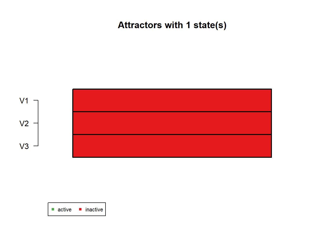
Attractor 1 is a simple attractor consisting of 1 state(s) and has a basin of 1 state(s):
|--<--|
V |
000 |
V |
|-->--|
Genes are encoded in the following order: V1 V2 V3
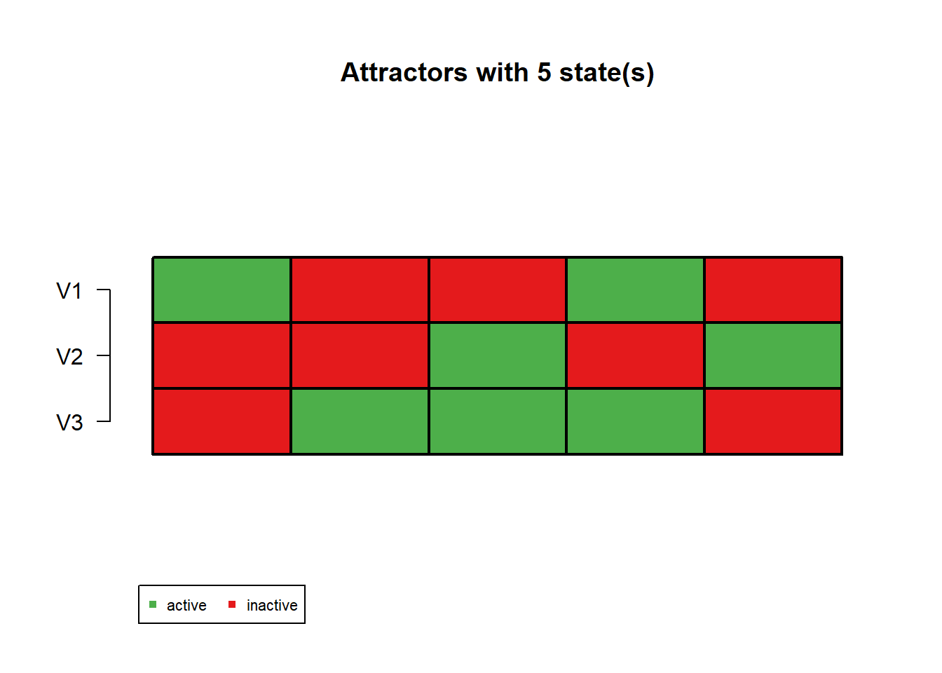
Attractor 2 is a simple attractor consisting of 5 state(s) and has a basin of 7 state(s):
|--<--|
V |
100 |
001 |
011 |
101 |
010 |
V |
|-->--|
Genes are encoded in the following order: V1 V2 V3
In the attractor plot, green means ON and red means OFF. The basin size tells you how many starting states eventually fall into that attractor.
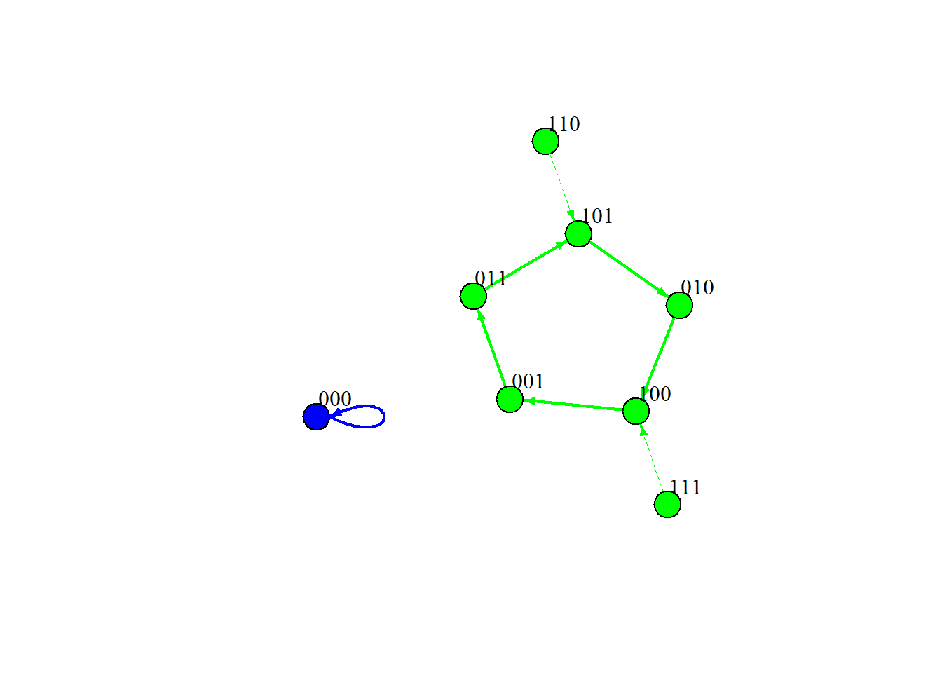
Interpretation of State Transition Graphs
Now that we have introduced attractors, it is important to note that attractors only become visible when we consider the entire state space/system.
As the system evolves over time, we will see that some paths move through the state space, other paths converge into a stable configuration (limit cycle), and other paths cycle indefinitely (fixed-point). This leads us to interpret attractor states and attractor basins.
All possible states of the system can be represented as tuples. For a two-node network, the states are \((0,0)\), \((0,1)\), \((1,0)\), and \((1,1)\). The transitions implied by the Boolean functions can be depicted as a state transition graph.
Continuing the example above:
From \((1,1)\), the system transitions to \((0,1)\).
From \((0,1)\), the system remains at \((0,1)\).
Thus, \((0,1)\) is a fixed-point attractor. The system also has fixed-point attractors at \((0,0)\) and \((1,0)\).
We can visualize the full state-transition graph for our simulated 3-node network like this:
Each node in the graph is a complete system state (e.g., 000). Arrows show where the system moves next under synchronous updating. Attractor states are the “sinks” that trap the dynamics.
Attractor desirability
So far, we’ve treated attractors as purely mathematical objects (stable configurations that emerge from the system’s update rules). But in research, we usually care about something more specific. Not all attractors are equally “good”. Some are desirable, others are undesirable.
Importantly, nothing in the math of Boolean networks labels an attractor as good or bad. A state like \((1,0,0)\) or \((1,1,1)\) is just a configuration of ON/OFF variables. It only becomes meaningful once we introduce domain knowledge.
So… how do we assign meaning to attractors? Researchers assign desirability to attractors using substantive knowledge about the system being modeled. This step is theory-driven.
In our depression example, states where depression (\(x_{1}\)) is OFF—such as \((0,0)\) and \((0,1)\)—are desirable, whereas the state \((1,0)\) (depression ON, adaptive coping behaviors are OFF) is undesirable. In other contexts, cancerous states or smoking behavior may be treated as undesirable attractors.
Student prompt: How do we decide whether an attractor is “useful” or desirable? Are attractors always clinically meaningful?
Network Control
Once attractors are extracted and labeled, the Boolean network framework supports the design of control strategies to move the system out of an undesirable attractor and toward a desirable one.
It is helpful to reframe the state transition graph as a space we can navigate:
Nodes = system states (e.g., 010, 111)
Edges = allowed transitions under the Boolean functions/update rules
Attractors = long-run stable endpoints (fixed points or limit cycles)
Attractor basins = regions of attraction
Over time, each trajectory eventually enters a basin and settles into an attractor. Based on all this information, we ask ourselves: How do we perturb the system so its trajectory moves from one undesirable basin into a desirable one?
A control strategy identifies a perturbation (often a temporary change to a node’s state or to its Boolean function) that pushes the system along the shortest path toward a desired attractor. A control strategy specifies three things:
Which node to intervene on (e.g., \(x_2\))
What value to set it to (e.g., force \(x_2\) = 1)
When/under what condition intervention occurs (i.e., only when system is in an undesirable attractor or basin)
This connects directly to the idea that Boolean networks are state-dependent and nonlinear: the effect of an intervention depends on the current configuration of the entire system.
Within the Boolean framework, control becomes a question of finding the shortest path to transition from an undesirable attractor basin to a state in a desirable basin. This is where calculating Hamming distance comes into play.
Hamming distance refers to the number of positions at which two binary systems differ.
Example: \((0,0,1)\) and \((1,0,0)\)
If we compare node by node, we see:
\(x_1\): 0 → 1 (difference of 1)
\(x_2\): 0 → 0 (difference of 0)
\(x_3\): 1 → 0 (difference of 1)
so, the Hamming distance between \((0,0,1)\) and \((1,0,0)\) is 2. This means two node interventions are required (at minimum) to transform one state into the other.
In the two-node depression example, one control strategy is to perturb \(x_{2}\) (turn adaptive coping behaviors ON) whenever \(x_{1}\) (depression) is ON. This moves the system from the undesirable attractor \((1,0)\) to \((1,1)\), and then to the desirable attractor \((0,1)\).
This induces the transition:
(1,0)→(1,1)→(0,1)
first, intervention breaks the undesirable equilibrium then system dynamics carry it into the desirable basin
Student prompt: What are the practical implications for designing an intervention? Can you think of a limitation (e.g., assuming we can perfectly manipulate one node without side effects)?
Methodological caveat: The provided context presents control as a search for shortest-path perturbations on the state transition graph. However, this assumes that the inferred Boolean functions are the “true” data-generating mechanism and that external perturbations can be implemented instantaneously and without cost—assumptions that may not hold in real-world psychological or biological systems.
Application: How to do this in \(\texttt{R}\)
Binarization of Continuous Data
Before fitting a Boolean network, continuous data must be binarized (e.g., via median splits, thresholds, or more sophisticated methods).
To see how this works in practice, we can simulate a noisy continuous time series from our known 3-node network and then binarize it:
# Simulate a single noisy time series from the known networkobserved =generateTimeSeries(network = net,numSeries =1, numMeasurements =500,type ="synchronous", noiseLevel =0.10)# Binarize the continuous observations back to 0/1 using k-means thresholdingbin_obj =binarizeTimeSeries(observed, method ="kmeans")bin = bin_obj$binarizedMeasurements# Convert to a standard matrix for network reconstructionbin_mat =as.matrix(bin[[1]][1,])# Compare the first few raw and binarized valuescbind(head(observed[[1]][1,], 10), head(bin_mat, 10))
Student prompt: When is binarization appropriate? What are the benefits and costs? Does binarization discard meaningful gradation in psychological data? Reference Yang et al. (2022) or Bertacchini et al. (2022) as needed.
Inference and implementation
There are two ways to infer Boolean functions:
Manual inference
When networks are very small (e.g., N=2 or N=3), we can sometimes manually derive Boolean rules by inspecting observed time series and identifying consistent logical patterns.
This involves reasoning through how combinations of inputs (via AND, OR, NOT) reproduce the observed transitions (which is very labor intensive)
Algorithmic inference
In practice, Boolean functions are typically inferred using algorithms that systematically search for the best-fitting logical rules.
Brute-force estimation procedure Boolean functions are inferred by comparing the observed time-series of each outcome variable \(x_{i}(t+1)\) with candidate functions built from input variables at time \(t\). The goal is to find the Boolean functions (logical rules) that best describe the temporal transitions of each node in a system based on observed binary time-series data.
Each candidate function is evaluated based on prediction error, typically defined as:
False positives (Type I error)
False negatives (Type II error)
The “best” function is the one that minimizes total error, balancing these two types of mistakes. This introduces a tradeoff between model fit and parsimony (simpler rules vs. overfitting).
The search proceeds across increasing values of \(K\) (the number of input variables allowed):
When \(K=1\): Each node depends on only one other node. The algorithm searches over constant functions and unary functions (e.g., \(x_{i}(t+1) = x_{i1}(t)\) or \(x_{i}(t+1) = \overline{x_{i1}(t)}\)), selecting the one with minimal error.
When \(K=2\): The algorithm searches over AND, OR, and NOT combinations of variable pairs, again selecting the function that minimizes prediction error (sum of false positives and false negatives).
When \(K > 2\): Recursive algorithms build upon the \(K=2\) case.
As \(K\) increases, the model flexibility increases, but the complexity grows exponentially. With that, the risk of overfitting also increases.
In practice, this can be implemented in \(\texttt{R}\) using the BoolNet package:
# Reconstruct Boolean functions from the binarized data# readableFunctions = TRUE shows rules in logic notation (e.g., !V2 & V3)recon =reconstructNetwork(bin, method ="bestfit",maxK = N -1,returnPBN =FALSE,readableFunctions =TRUE)recon
Probabilistic Boolean network with 3 genes

Involved genes:
V1 V2 V3

Transition functions:

Alternative transition functions for gene V1:
V1 = (V2) (error: 0)

Alternative transition functions for gene V2:
V2 = (!V2 & V3) (error: 0)

Alternative transition functions for gene V3:
V3 = (!V1 & V3) | (V1 & !V3) (error: 0)
Next, we choose a single deterministic realization from the reconstruction and compare synchronous versus asynchronous updating:
# Choose a single deterministic realizationsinglenet =chooseNetwork(recon, functionIndices =rep(1, N),dontCareValues =rep(1, N),readableFunctions =TRUE)# Synchronous update: all nodes update simultaneouslyga =getAttractors(network = singlenet, type ="synchronous",returnTable =TRUE)ga
Attractor 1 is a simple attractor consisting of 1 state(s) and has a basin of 1 state(s):

 |--<--|
 V     |
 000   |
 V     |
 |-->--|


Genes are encoded in the following order: V1 V2 V3

Attractor 2 is a simple attractor consisting of 5 state(s) and has a basin of 7 state(s):

 |--<--|
 V     |
 100   |
 001   |
 011   |
 101   |
 010   |
 V     |
 |-->--|


Genes are encoded in the following order: V1 V2 V3
# Asynchronous update: one randomly selected node updates at each stepga2 =getAttractors(network = singlenet, type ="asynchronous")ga2
Attractor 1 is a simple attractor consisting of 1 state(s):

 |--<--|
 V     |
 000   |
 V     |
 |-->--|


Genes are encoded in the following order: V1 V2 V3
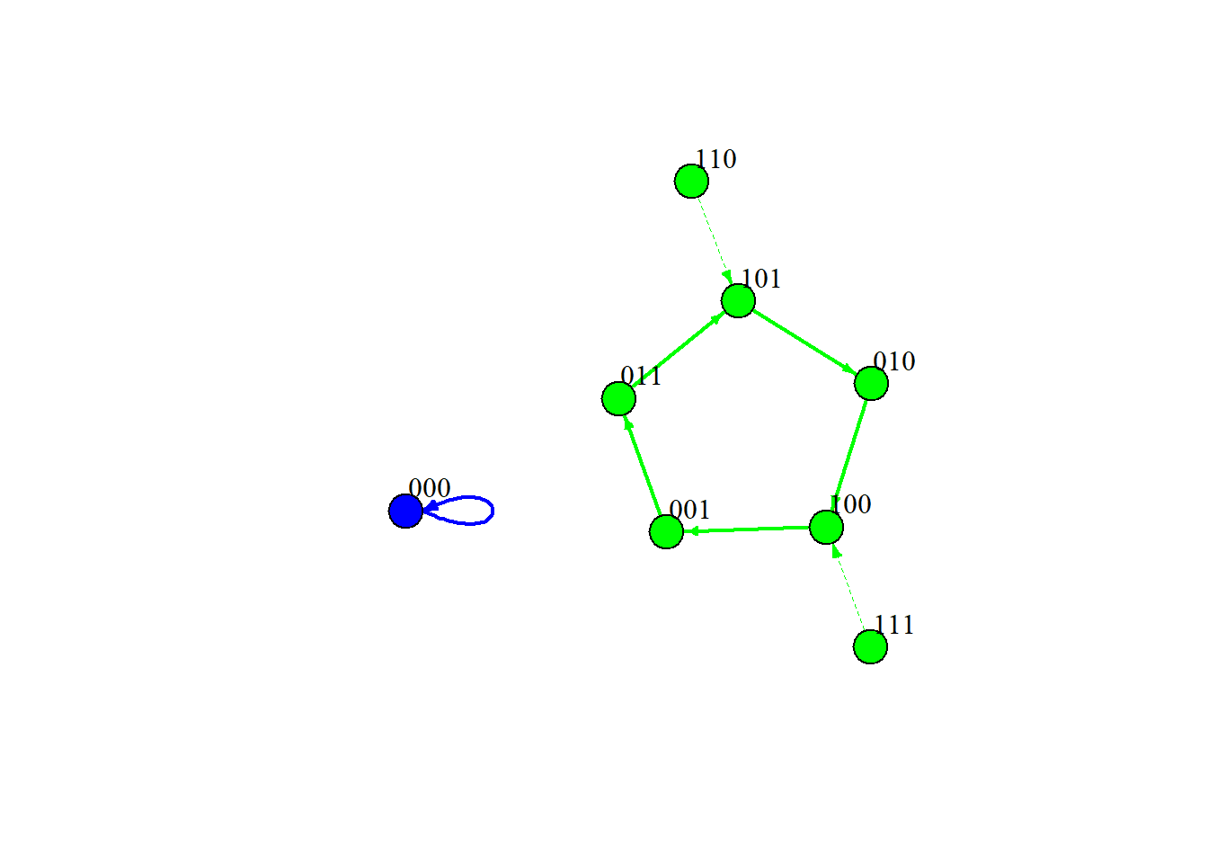
Finally, we can plot the state transition graph of the reconstructed network:
Notice that synchronous updating usually yields simple fixed-point or cyclic attractors, whereas asynchronous updating can reveal “loose” or complex attractors. In real psychological data, the timing of updates is rarely perfectly simultaneous, so this distinction matters.
Reflection/Discussion Questions
Boolean networks were originally developed for gene regulatory networks. What changes—if any—are needed to apply them to psychological time-series?
What are the limitations of assuming synchronous updating (all nodes update at once) versus asynchronous updating?
The state space grows as \(2^{N}\). What does this imply for scalability as the number of nodes \(N\) increases?
How does the Boolean network approach compare to the Ising model for binary data?
Campbell and Albert (2019) discuss “edgetic” perturbations (modifying single regulatory edges rather than knocking out whole nodes). How does this refine the concept of network control?