Continuous Data: Where variables are being measured on an interval and can be seen as a range, and we see in dynamic networks.
Weighted Data: the observation of the strength in relationships and help us to model the systems in the real world.
Time Series Data: Using variables as predictions and the repeated measurements collected over an amount of time (built with models like VAR covered last week)
Categorical Data: variables put into discrete categories
Regular graphs are binary {0,1}
Remember G=(V,E) \(\rightarrow\) where V represents the nodes and E represents the edges
The adjacency matrix A for binary graphs shows if nodes i and j are connected as 1; otherwise it is represented by 0
We can trivially extend this to continuous data
The binary graph only takes in the presence or absence of a relationship but with the continuous data we are adding real values, and these edges contain either the strength, magnitude or the direction of the relationships referring to the data being weighted
Weighted Network Examples
Degree \(\rightarrow\) Strength
A good example that we can look at are Transportation Networks: the edges in this case show the traffic flow and the degree becomes strength
Another example is that of symptoms where the edges have strength, a symptom can have more of a severity on others
Models of continuous data are much easier to imagine in psychology:
Partial Correlation Networks
Dynamic Networks
Etc.
The analysis of binary data is more difficult: - Ising model for cross-sectional data - Not a clear dynamic model for binary data
Thus, here is the gap filled by Boolean networks, which can model dynamical systems with binary states.
Boolean Networks
Think of the Boolean Network as a way to model time series: we are gathering many of the 1’s and 0’s to analyze the behavior of a system
In this section let us learn how to count in binary and the rules of this network
Discuss binary data
i.e., How are integers counted in binary
For example, 000 to 111
000 = 0
001 = 1
010 = 2
011 = 3
100 = 4
101 = 5
110 = 6
111 = 7
Describe Boolean rules
Boolean networks operate on three fundamental operators:
AND rules (\(\wedge\)): The outcome is ON only if all inputs are ON.
OR rules (\(\vee\)): The outcome is ON if any input is ON.
NOT rules (\(\overline{x}\)): The outcome is the opposite of the input.
\(x(t)\)
\(y(t)\)
\(x(t) \wedge y(t)\)
0
0
0
0
1
0
1
0
0
1
1
1
\(x(t)\)
\(y(t)\)
\(x(t) \vee y(t)\)
0
0
0
0
1
1
1
0
1
1
1
1
\(x(t)\)
\(\overline{x(t)}\)
0
1
1
0
Table recreated from Yang et al. (2022).
Describe the Boolean Network Model
Formulation
A Boolean network \(G(X, B)\) is defined by a set of nodes \(X = \{x_{1}, x_{2}, \dots, x_{n}\}\) and a set of Boolean functions \(B = \{f_{1}, f_{2}, \dots, f_{n}\}\).
When \(x_{i}(t) = 1\), the node is activated (ON) at time \(t\); when \(x_{i}(t) = 0\), the node is dormant (OFF). The vector \(X(t)\) describes the current state of the system, and the Boolean functions describe the dynamics—specifically, how the states change from \(X(t)\) to \(X(t+1)\).
where \(k\) specific input nodes determine the state of \(x_{i}\) at the next time step. The operators inside \(f_{i}\) can be any combination of AND, OR, and NOT.
A concrete two-node example
Consider a system with nodes \(x_{1}\) and \(x_{2}\). The following Boolean functions might be inferred from observed binary time-series:
Interpretation: \(x_{1}\) at time \(t+1\) depends on \(x_{1}\) and the negation of \(x_{2}\) at time \(t\). If \(x_{2}\) is ON, \(x_{1}\) turns OFF. Meanwhile, \(x_{2}\) simply persists in its previous state.
Student prompt: Lets use the example that we see a lot in coming of age movies and the expected experience that can happen in college. Referring to peers, risktaking and not being monitored by parents.
Let us denote the risk taking as: risktaking(t+1); peerrisktaking(t); and -parental monitoring(t)
Time to break this down: Our risk taking is ON only if our peers are being risk takers AND our parents are not monitoring.
Nonlinearity
When a Boolean function contains two variables connected with an AND operator, it acts like multiplication: the outcome is 1 only when both inputs are 1. Because \(z = x \wedge y\) behaves similarly to \(z = x \cdot y\), the AND operator captures nonlinear interactions. The combination of AND with NOT allows the expression of propositional first-order logic for nonlinear dynamics.
Attractors
What are attractors in dynamical systems?
Attractors indicate the long-term behavior of a system—areas of the phase space that the system occupies or approaches more frequently than others. There are many types:
Fixed-point attractor: The system settles to a single state and remains there.
Limit cycle attractor: The system cycles through a set of states repeatedly.
Multi-stability: Nonlinear systems can have multiple attractors, meaning they may get “stuck” in different persistent patterns depending on initial conditions.
In code, we can build a small random Boolean network and extract its attractors to see these patterns concretely:
N =3net =generateRandomNKNetwork(n = N, k =2, topology ="homogeneous", linkage ="uniform", functionGeneration ="uniform",noIrrelevantGenes =FALSE, simplify =TRUE)net$genes =paste0("V", 1:N)Attractors =getAttractors(net)plotAttractors(Attractors)
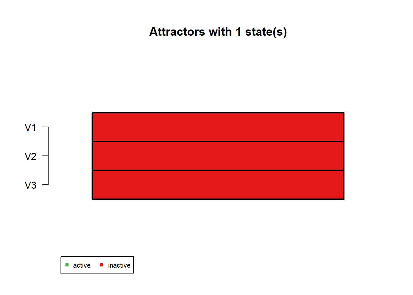
Attractor 1 is a simple attractor consisting of 1 state(s) and has a basin of 1 state(s):
|--<--|
V |
000 |
V |
|-->--|
Genes are encoded in the following order: V1 V2 V3
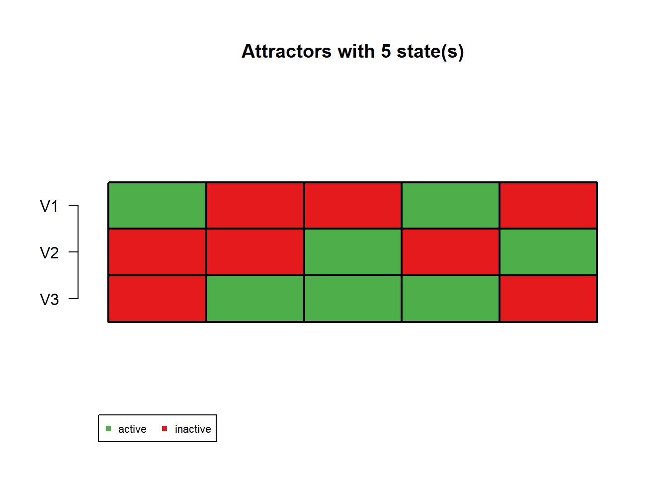
Attractor 2 is a simple attractor consisting of 5 state(s) and has a basin of 7 state(s):
|--<--|
V |
100 |
001 |
011 |
101 |
010 |
V |
|-->--|
Genes are encoded in the following order: V1 V2 V3
In the attractor plot, green means ON and red means OFF. The basin size tells you how many starting states eventually fall into that attractor.
Interpretation of State Transition Graphs
All possible states of the system can be represented as tuples. For a two-node network, the states are \((0,0)\), \((0,1)\), \((1,0)\), and \((1,1)\). The transitions implied by the Boolean functions can be depicted as a state transition graph.
Continuing the example above:
From \((1,1)\), the system transitions to \((0,1)\).
From \((0,1)\), the system remains at \((0,1)\).
Thus, \((0,1)\) is a fixed-point attractor. The system also has fixed-point attractors at \((0,0)\) and \((1,0)\).
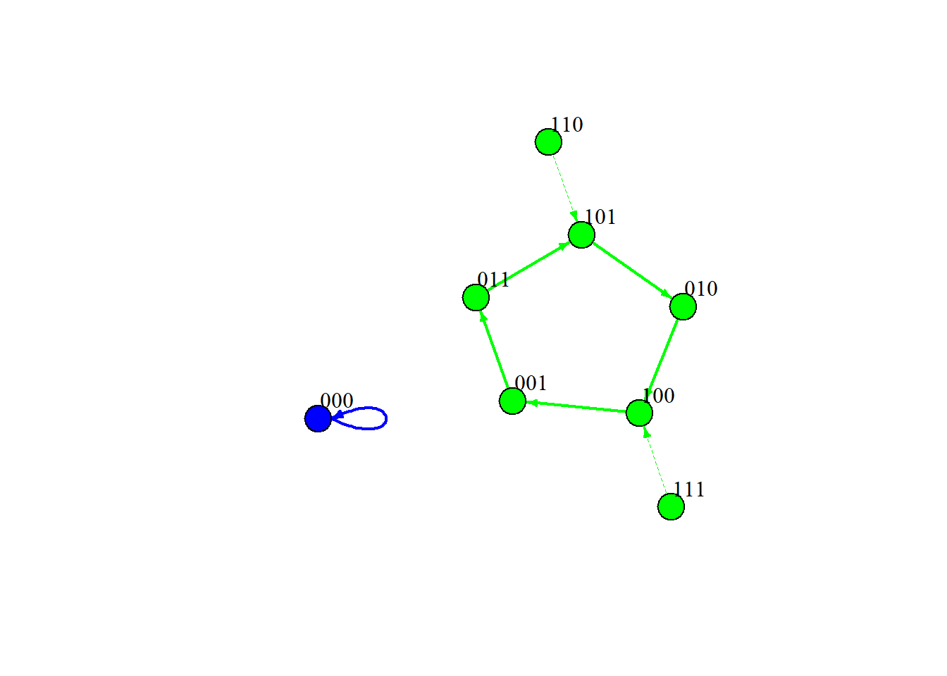
We can visualize the full state-transition graph for our simulated 3-node network like this:
Each node in the graph is a complete system state (e.g., 000). Arrows show where the system moves next under synchronous updating. Attractor states are the “sinks” that trap the dynamics.
Student prompt: Draw or describe the state transition graph for your chosen example. What are the attractors? Are they fixed points or limit cycles?
Attractor desirability
Researchers use domain knowledge to classify attractors as desirable or undesirable. For instance, in the emotion regulation example, states where anger (\(x_{1}\)) is OFF—such as \((0,0)\) and \((0,1)\)—are desirable, whereas the state \((1,0)\) (anger ON, distraction OFF) is undesirable. In other contexts, cancerous states or smoking behavior may be treated as undesirable attractors.
Student prompt: How do we decide whether an attractor is “useful” or desirable? Are attractors always clinically meaningful?
Network Control
Once attractors are extracted and labeled, the Boolean network framework supports the design of control strategies to move the system out of an undesirable attractor and toward a desirable one.
A control strategy identifies a perturbation—often a temporary change to a node’s state or to its Boolean function—that pushes the system along the shortest path toward a desired attractor. In the two-node example, one control strategy is to perturb \(x_{2}\) (turn distraction ON) whenever \(x_{1}\) (anger) is ON. This moves the system from the undesirable attractor \((1,0)\) to \((1,1)\), and then to the desirable attractor \((0,1)\).
Student prompt: Explain the logic of network control in your own words. What are the practical implications for designing an intervention? Can you think of a limitation (e.g., assuming we can perfectly manipulate one node without side effects)?
Methodological caveat: The provided context presents control as a search for shortest-path perturbations on the state transition graph. However, this assumes that the inferred Boolean functions are the “true” data-generating mechanism and that external perturbations can be implemented instantaneously and without cost—assumptions that may not hold in real-world psychological or biological systems.
Application: How to do this in \(\texttt{R}\)
Binarization of Continuous Data
Before fitting a Boolean network, continuous data must be binarized (e.g., via median splits, thresholds, or more sophisticated methods).
To see how this works in practice, we can simulate a noisy continuous time series from our known 3-node network and then binarize it:
# Simulate a single noisy time series from the known networkobserved =generateTimeSeries(network = net,numSeries =1, numMeasurements =500,type ="synchronous", noiseLevel =0.10)# Binarize the continuous observations back to 0/1 using k-means thresholdingbin_obj =binarizeTimeSeries(observed, method ="kmeans")bin = bin_obj$binarizedMeasurements# Convert to a standard matrix for network reconstructionbin_mat =as.matrix(bin[[1]][1,])# Compare the first few raw and binarized valuescbind(head(observed[[1]][1,], 10), head(bin_mat, 10))
Student prompt: When is binarization appropriate? What are the benefits and costs? Does binarization discard meaningful gradation in psychological data? Reference Yang et al. (2022) or Bertacchini et al. (2022) as needed.
Inference and implementation
The Boolean functions are inferred by comparing the observed time-series of each outcome variable \(x_{i}(t+1)\) with candidate functions built from input variables at time \(t\). The search proceeds across increasing values of \(K\) (the number of input variables allowed):
When \(K=1\): The algorithm searches over constant functions and unary functions (e.g., \(x_{i}(t+1) = x_{i1}(t)\) or \(x_{i}(t+1) = \overline{x_{i1}(t)}\)), selecting the one with minimal error.
When \(K=2\): The algorithm searches over AND, OR, and XOR combinations of variable pairs, again selecting the function that minimizes prediction error (sum of false positives and false negatives).
When \(K > 2\): Recursive algorithms build upon the \(K=2\) case.
In practice, this can be implemented in \(\texttt{R}\) using the BoolNet package:
# Reconstruct Boolean functions from the binarized data# readableFunctions = TRUE shows rules in logic notation (e.g., !V2 & V3)recon =reconstructNetwork(bin, method ="bestfit",maxK = N -1,returnPBN =FALSE,readableFunctions =TRUE)recon
Probabilistic Boolean network with 3 genes

Involved genes:
V1 V2 V3

Transition functions:

Alternative transition functions for gene V1:
V1 = (V2) (error: 0)

Alternative transition functions for gene V2:
V2 = (!V2 & V3) (error: 0)

Alternative transition functions for gene V3:
V3 = (!V1 & V3) | (V1 & !V3) (error: 0)
Next, we choose a single deterministic realization from the reconstruction and compare synchronous versus asynchronous updating:
# Choose a single deterministic realizationsinglenet =chooseNetwork(recon, functionIndices =rep(1, N),dontCareValues =rep(1, N),readableFunctions =TRUE)# Synchronous update: all nodes update simultaneouslyga =getAttractors(network = singlenet, type ="synchronous",returnTable =TRUE)ga
Attractor 1 is a simple attractor consisting of 1 state(s) and has a basin of 1 state(s):

 |--<--|
 V     |
 000   |
 V     |
 |-->--|


Genes are encoded in the following order: V1 V2 V3

Attractor 2 is a simple attractor consisting of 5 state(s) and has a basin of 7 state(s):

 |--<--|
 V     |
 100   |
 001   |
 011   |
 101   |
 010   |
 V     |
 |-->--|


Genes are encoded in the following order: V1 V2 V3
# Asynchronous update: one randomly selected node updates at each stepga2 =getAttractors(network = singlenet, type ="asynchronous")ga2
Attractor 1 is a simple attractor consisting of 1 state(s):

 |--<--|
 V     |
 000   |
 V     |
 |-->--|


Genes are encoded in the following order: V1 V2 V3
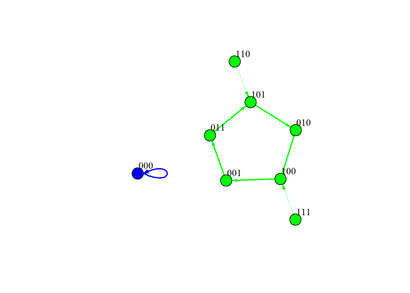
Finally, we can plot the state transition graph of the reconstructed network:
Notice that synchronous updating usually yields simple fixed-point or cyclic attractors, whereas asynchronous updating can reveal “loose” or complex attractors. In real psychological data, the timing of updates is rarely perfectly simultaneous, so this distinction matters.
Reflection/Discussion Questions
Boolean networks were originally developed for gene regulatory networks. What changes—if any—are needed to apply them to psychological time-series?
What are the limitations of assuming synchronous updating (all nodes update at once) versus asynchronous updating?
The state space grows as \(2^{N}\). What does this imply for scalability as the number of nodes \(N\) increases?
How does the Boolean network approach compare to the Ising model or Markov chain methods for binary data?
Campbell and Albert (2019) discuss “edgetic” perturbations (modifying single regulatory edges rather than knocking out whole nodes). How does this refine the concept of network control?