Dr. Park’s Community Detection
What are Communities?
In the real-world, understanding how variables or people group or “cluster” together can be a helpful heuristic tool for summarizing large amounts of data.
For example, we can survey a vast array of individuals and measure their specific political interests and beliefs.
What we would find is that many people have quite idiosyncratic and complex beliefs and values. However, we may also conjecture that the broader political party you register with and support probably describes–on average–most of your beliefs and values with an acceptable degree of accuracy. This is to say, groups or clusters of individuals by political party registration is a decent approximation of your underlying beliefs and morals. Not perfect but decent enough.
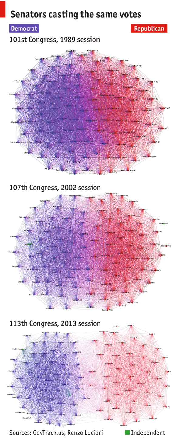
For example, in the above image, we can see that there are 2 communities. This may be due to the coloration but also–in the latter sessions of the US congress, we can definitely see a clear separation forming.
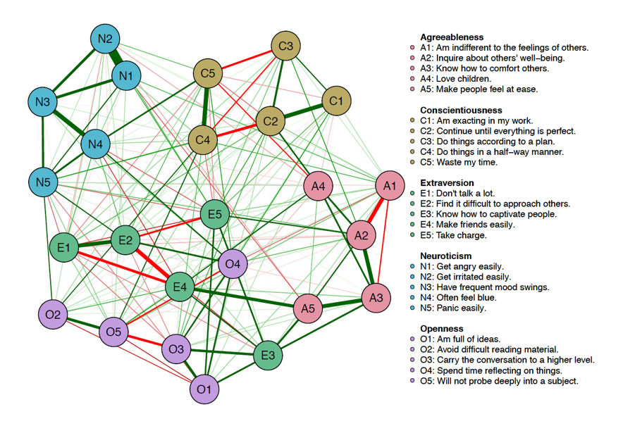
Likewise, in the field of psychology, we often make use of community detection methods to identify clusters of variables (e.g., people, symptoms, genes) which are more akin to one another than they are to variables in other groups. For instance, we may think of psychological disorders as being comprised of their psychological symptoms; however, we know\(^{*}\) that certain symptoms tend to coalesce with others. That is, symptoms of depression probably interact with other symptoms of depression more than they do with symptoms of post-traumatic stress disorder (PTSD). Alernatively, we may expect that survey items that measure dimensions of personality will “hang” together as in the below image.
In another example, we may imagine that regions of the brain may form communities or clusters based on what systems they govern: the Hypothalamic-Pituitary-Adrenal (HPA) axis is often implicated in stress response and regulation in individuals. Thus, we may expect that components of that system: the hypothalamus, the pituitary gland, and the adrenal glands may be interconnected to one another.
This is to say, communities or groups likely exist in many areas of scientific inquiry.
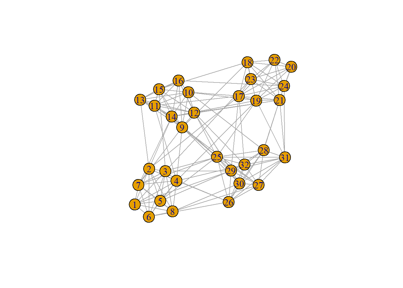
The goal of this week’s tutorial is to walk folks through an implementation of some clustering methods to a hypothetical dataset comprised of multiple individuals who may have sub-types of depression. We may–for example–have an adjacency matrix that encodes the number of symptoms they share with one another.
From the plot above, we can see that there appear to be 4-clusters of individuals; however, the challenge is determining whether this observation is supported in some way.
Let’s take a look at our data:
adjacency.matrix [,1] [,2] [,3] [,4] [,5] [,6] [,7] [,8] [,9] [,10] [,11] [,12] [,13]
[1,] 0 2 3 2 3 2 2 3 0 0 0 0 0
[2,] 2 0 4 3 2 2 1 2 0 0 0 0 1
[3,] 3 4 0 1 2 3 2 3 0 0 0 0 0
[4,] 2 3 1 0 2 3 3 2 1 0 1 0 0
[5,] 3 2 2 2 0 2 3 2 0 0 0 0 0
[6,] 2 2 3 3 2 0 2 4 0 0 0 0 0
[7,] 2 1 2 3 3 2 0 3 1 0 0 0 0
[8,] 3 2 3 2 2 4 3 0 0 0 0 0 0
[9,] 0 0 0 1 0 0 1 0 0 1 1 2 3
[10,] 0 0 0 0 0 0 0 0 1 0 3 3 3
[11,] 0 0 0 1 0 0 0 0 1 3 0 3 4
[12,] 0 0 0 0 0 0 0 0 2 3 3 0 3
[13,] 0 1 0 0 0 0 0 0 3 3 4 3 0
[14,] 0 1 0 0 0 0 1 0 2 2 3 3 2
[15,] 0 0 1 0 0 0 0 0 3 3 2 3 4
[16,] 0 0 0 0 0 0 0 0 2 2 2 2 3
[17,] 0 1 0 0 0 0 0 0 0 1 1 0 0
[18,] 0 0 0 0 0 0 0 0 1 0 0 0 0
[19,] 0 0 0 1 0 0 0 0 0 1 0 0 0
[20,] 0 0 0 0 0 0 0 0 0 0 0 0 0
[21,] 0 0 0 0 0 0 0 0 0 0 0 1 0
[22,] 0 0 0 0 0 0 0 0 0 0 0 0 0
[23,] 0 0 1 0 0 0 0 0 0 0 0 0 0
[24,] 0 0 0 0 0 0 0 0 0 0 0 0 0
[25,] 0 0 1 0 1 0 1 0 1 0 0 0 0
[26,] 0 1 0 1 0 1 0 0 0 0 0 0 0
[27,] 0 0 0 0 0 0 0 1 1 0 0 0 0
[28,] 0 0 0 0 0 0 0 0 0 1 0 0 0
[29,] 1 0 1 0 0 0 0 0 0 0 0 1 0
[30,] 0 0 0 0 0 0 0 1 1 0 0 1 0
[31,] 0 0 0 0 0 0 0 0 0 0 0 0 0
[32,] 0 0 0 1 1 0 0 0 0 0 0 1 0
[,14] [,15] [,16] [,17] [,18] [,19] [,20] [,21] [,22] [,23] [,24] [,25]
[1,] 0 0 0 0 0 0 0 0 0 0 0 0
[2,] 1 0 0 1 0 0 0 0 0 0 0 0
[3,] 0 1 0 0 0 0 0 0 0 1 0 1
[4,] 0 0 0 0 0 1 0 0 0 0 0 0
[5,] 0 0 0 0 0 0 0 0 0 0 0 1
[6,] 0 0 0 0 0 0 0 0 0 0 0 0
[7,] 1 0 0 0 0 0 0 0 0 0 0 1
[8,] 0 0 0 0 0 0 0 0 0 0 0 0
[9,] 2 3 2 0 1 0 0 0 0 0 0 1
[10,] 2 3 2 1 0 1 0 0 0 0 0 0
[11,] 3 2 2 1 0 0 0 0 0 0 0 0
[12,] 3 3 2 0 0 0 0 1 0 0 0 0
[13,] 2 4 3 0 0 0 0 0 0 0 0 0
[14,] 0 2 1 0 0 1 0 1 0 0 0 1
[15,] 2 0 2 0 1 0 0 0 0 0 0 0
[16,] 1 2 0 0 0 0 0 0 0 0 1 1
[17,] 0 0 0 0 3 2 2 1 3 3 3 0
[18,] 0 1 0 3 0 2 4 1 4 1 2 0
[19,] 1 0 0 2 2 0 3 1 3 3 3 1
[20,] 0 0 0 2 4 3 0 2 1 2 4 0
[21,] 1 0 0 1 1 1 2 0 3 1 1 0
[22,] 0 0 0 3 4 3 1 3 0 2 1 0
[23,] 0 0 0 3 1 3 2 1 2 0 1 0
[24,] 0 0 1 3 2 3 4 1 1 1 0 0
[25,] 1 0 1 0 0 1 0 0 0 0 0 0
[26,] 0 0 0 0 0 0 0 0 0 0 0 1
[27,] 0 0 0 0 0 0 0 0 0 0 0 3
[28,] 0 0 0 0 0 0 0 1 0 0 1 2
[29,] 0 0 0 1 0 0 0 0 0 0 0 3
[30,] 0 0 0 0 0 0 0 0 0 0 0 2
[31,] 0 0 0 0 0 1 0 1 0 0 1 1
[32,] 0 0 0 1 0 0 0 0 0 0 0 3
[,26] [,27] [,28] [,29] [,30] [,31] [,32]
[1,] 0 0 0 1 0 0 0
[2,] 1 0 0 0 0 0 0
[3,] 0 0 0 1 0 0 0
[4,] 1 0 0 0 0 0 1
[5,] 0 0 0 0 0 0 1
[6,] 1 0 0 0 0 0 0
[7,] 0 0 0 0 0 0 0
[8,] 0 1 0 0 1 0 0
[9,] 0 1 0 0 1 0 0
[10,] 0 0 1 0 0 0 0
[11,] 0 0 0 0 0 0 0
[12,] 0 0 0 1 1 0 1
[13,] 0 0 0 0 0 0 0
[14,] 0 0 0 0 0 0 0
[15,] 0 0 0 0 0 0 0
[16,] 0 0 0 0 0 0 0
[17,] 0 0 0 1 0 0 1
[18,] 0 0 0 0 0 0 0
[19,] 0 0 0 0 0 1 0
[20,] 0 0 0 0 0 0 0
[21,] 0 0 1 0 0 1 0
[22,] 0 0 0 0 0 0 0
[23,] 0 0 0 0 0 0 0
[24,] 0 0 1 0 0 1 0
[25,] 1 3 2 3 2 1 3
[26,] 0 1 1 3 2 1 2
[27,] 1 0 3 3 4 2 1
[28,] 1 3 0 3 2 2 2
[29,] 3 3 3 0 2 3 3
[30,] 2 4 2 2 0 1 3
[31,] 1 2 2 3 1 0 2
[32,] 2 1 2 3 3 2 0range(adjacency.matrix)[1] 0 4It appears that our subjects have anywhere between 0 and 4 symptoms in common with one another. We probably expect people who share many symptoms with one another to form communities.
Now comes the challenge.
Defining a Community
We begin by asking this question. What is a community? How do I know that things are more similar to one another within a group but dissimilar with other groups? In the real world, we find it quite easy to draw lines that separate groups or people or other things. The question in this case, is more focused on whether or not we can define–mathematically–what makes a community a community.
We begin by describing an “objective function”. Often, we are not sure whether there is a true, analytic solution to a given problem. Instead, we will define some function of our data that–if optimized–produces an answer or solution that we believe. We will find that today’s lecture on community detection methods leans heavily on these objective functions.
The first objective function that we’ll cover is the following:
\[J(X) = \sum_{j=1}^{C} \sum_{i=1}^{n_{j}} ||x_{i} - \bar{\mathbf{x}}_j ||^{2}\] This equation is what one might use as an objective function to define who/what belongs in which group for a specified number of groups, \(k\). We can break this equation down into simpler components and language.
- \(J(\mathbf{X})\) is our function that depends on inputs, \(\mathbf{X}\)
- The inner component of the sums: \(||\mathbf{x}_{i} - \bar{\mathbf{x}}_{j}||\) is calculating the distance between the \(i^{th}\) data point[s] and the mean of the \(j^{th}\) community[ies]
- This term is the deviations of our data from what we’ll henceforth refer to as the “centroids” of our data
- \(||\cdot ||^{2}\) represents the squared Euclidean distances
- \(\sum_{i=1}^{n_{j}}\) is the sum from the first to the number of individuals in the \(j^{th}\) community
- \(\sum_{j=1}^{C}\) is the sum from the first to the \(C^{th}\) community
In sum, this objective function produces a value that represents the sum of squared deviations from each individual to each group.
Now, we can think on this a little bit. If we assign people to groups correctly do we expect individuals to be closer or further from their group means/averages?
Answer.
We probably want individuals to be closer to their group averages.
That is, if we are putting people into groups and we want our groups to be good descriptions of the individuals in them, it helps if our groups are homogeneous rather than heterogeneous. Thus, we’d prefer individual scores \(\mathbf{x}_{i}\) to be close to the group score, \(\bar{\mathbf{x}}_{j}\)
So, based on our observation of this objective function, it might do the job of fitting people into groups if we minimize the function. That is, we try to find an arrangement of our \(N\) variables such that they fall into \(C\) or \(k\) communities.
\(k\)-means Clustering
\(k\)-means Clustering is one approach that we can use–coupled with the objective function described above to accomplish this. What \(k\)-means does is the following:
- Randomly assign individuals to \(k\) groups
- Calculate the “centroid” or means of each group and assess the objective function \(J(\mathbf{X})\)
- “Shuffle” individuals such that they move to other clusters whose centroids they are closer to
- Repeat the second and third step until subjects no longer substantially shift in their positions over time
We can do most of this in an automated way in \(\texttt{R}\). First, we’ll load all the packages we’ll need for today.
library(igraph)
library(stats)
library(mclust)
Package 'mclust' version 6.1.1
Type 'citation("mclust")' for citing this R package in publications.library(ppclust)Then, we can begin work on the \(k\)-means clustering approach.
Below, you’ll see code for running the \(k\)-means algorithm on our adjacency matrix. Each argument can be described as:
- \(\texttt{centers}\): How many communites do we think there are?
- \(\texttt{iter.max}\): How many times should we allow \(k\)-means to shuffle people before stopping [if it doesn’t stop before then]
- \(\texttt{nstart}\): How many times should we randomly put people into groups
Now, why do we need to start \(30\) times?
Answer.
Recall how the algorithm works. We begin by randomly placing people into groups to start. This random placement could influence how we shuffle people at each step. To ensure our solution is “robust” we add multiple starts and take the solution that is most stable.
solution1 = kmeans(adjacency.matrix,
                   centers = 3,
                   iter.max = 1000,
                   nstart = 30)
solution1$cluster
[1] 3 3 3 3 3 3 3 3 1 1 1 1 1 1 1 1 2 2 2 2 2 2 2 2 2 2 2 2 2 2 2 2solution1$tot.withinss[1] 582.0625Once we run the code we get output such as \(\texttt{solution1\$cluster}\). This contains the group assignments. As we can see, it looks like it put the first 8 people into a group.
We also get a value called the “total within-cluster sums of squares”. In a way, this is telling us the total amount of “error” with our solution. Now, with clustering approaches that optimize \(J(\mathbf{X})\) we often see an interesting behavior which is that our total within-cluster sums of squares always decreases with the more clusters we extract.
Why might that be?
Answer.
If we take this to the extreme end and just put people into their own clusters then the distance between a person and their own mean is \(0.00\). There’s no error when you’re in a group by yourself. So, technically, the best solution to the function \(J(\mathbf{X})\) is to just put people into their own groups.
Problem solved, right?
Well, yes and no. Yes because that’s the optimal solution but also no because we want groups that provide general utility even if they can be slightly wrong at times. So, a better way of approaching this would be to define a group as when we’ve made the most improvement to the within-cluster sums of squares but without overdoing it.
To demonstrate how within-cluster sums of squares always decreases, we can plot the error as we extract more and more groups.
The code below will extract 1 to \(\texttt{round(((n.nodes.per.group*n.groups)/3)}\) groups. In this case, I know the answer so I coded that in. But I am basically saying generate 1 to the total number of people divided by 3 or \(\frac{N}{3}\). This is just to demonstrate the behavior of within-cluster error so I am not going to extract all \(N\) solutions:
results.1 = lapply(1:round(((n.nodes.per.group*n.groups)/3)),
                   function(k) kmeans(adjacency.matrix,
                                      centers = k,
                                      iter.max = 1000,
                                      nstart = 30))
wss.vals = sapply(results.1, function(res) sum(res$withinss))
plot(wss.vals, type = "l")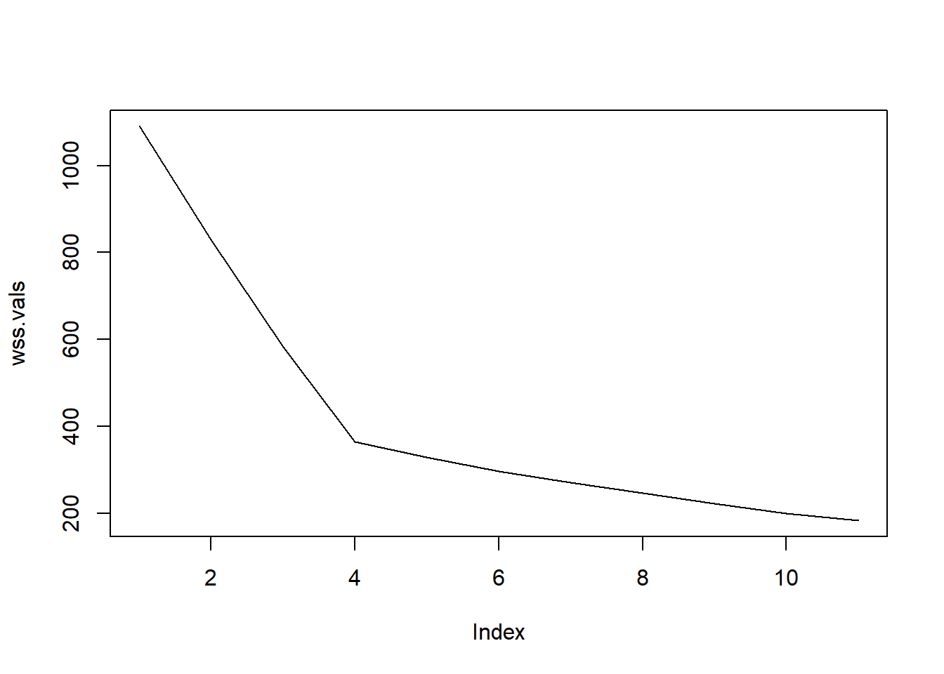
Based on the plot above, what number of clusters or groups seems most appropriate to you? How do you know? Or why do you feel that way?
The plot above can be referred to as a “scree plot” and shows how the within-cluster sums of squares always goes down with each community we extract. Remember, if everyone is in a cluster by themselves, there’s no error. In this case, we might choose to say that 4-groups is the best answer because the rate at which within-cluster sums of squares changes, slows down after that point.
Alternatively, we can think of it as “finding the elbow” in the scree plot. Now, this approach isn’t perfect but it can often be generally quite decent.
So, based on this, we find that there are 4-groups of individuals each comprised of 8-individuals. Let’s revisit the adjacency matrix but focus solely on one area of it:
adjacency.matrix[1:16, 1:16] [,1] [,2] [,3] [,4] [,5] [,6] [,7] [,8] [,9] [,10] [,11] [,12] [,13]
[1,] 0 2 3 2 3 2 2 3 0 0 0 0 0
[2,] 2 0 4 3 2 2 1 2 0 0 0 0 1
[3,] 3 4 0 1 2 3 2 3 0 0 0 0 0
[4,] 2 3 1 0 2 3 3 2 1 0 1 0 0
[5,] 3 2 2 2 0 2 3 2 0 0 0 0 0
[6,] 2 2 3 3 2 0 2 4 0 0 0 0 0
[7,] 2 1 2 3 3 2 0 3 1 0 0 0 0
[8,] 3 2 3 2 2 4 3 0 0 0 0 0 0
[9,] 0 0 0 1 0 0 1 0 0 1 1 2 3
[10,] 0 0 0 0 0 0 0 0 1 0 3 3 3
[11,] 0 0 0 1 0 0 0 0 1 3 0 3 4
[12,] 0 0 0 0 0 0 0 0 2 3 3 0 3
[13,] 0 1 0 0 0 0 0 0 3 3 4 3 0
[14,] 0 1 0 0 0 0 1 0 2 2 3 3 2
[15,] 0 0 1 0 0 0 0 0 3 3 2 3 4
[16,] 0 0 0 0 0 0 0 0 2 2 2 2 3
[,14] [,15] [,16]
[1,] 0 0 0
[2,] 1 0 0
[3,] 0 1 0
[4,] 0 0 0
[5,] 0 0 0
[6,] 0 0 0
[7,] 1 0 0
[8,] 0 0 0
[9,] 2 3 2
[10,] 2 3 2
[11,] 3 2 2
[12,] 3 3 2
[13,] 2 4 3
[14,] 0 2 1
[15,] 2 0 2
[16,] 1 2 0By taking the first 16 rows and columns, we should be seeing the first 2 groups and their data. From looking at the matrix, can you see the groups?
Answer.
We can notice that the first \(8\times 8\) portion of the matrix has numbers ranging from 1- to 4-symptoms. But if we look at rows \(9:16\) and columns \(1:8\), we see mostly 0’s and some 1’s. This seems to suggest that the first 8 people do not tend to share a lot of symptoms in common with the second 8 people.
Great, so we’ve successfully run \(k\)-means clustering on our data. We found 4-subgroups of people who share psychological symptoms.
But how confident are we that people belong to the groups we assigned them to? Put another way, if we were \(52\%\) sure that someone belonged to a group, would you be willing to assign them to that group? What degree of confidence would you need to assign someone to a group?
Fuzzy \(c\)-means Clustering
This idea, that group assignments have ambiguity is not novel by any means. As we discussed earlier, we form groups because they are heuristically useful not because they are always true and correct.
\(k\)-means has several weaknesses but one of the primary weaknesses is that it will confidently give you \(k\)-groups if you ask for it. Determining whether a particular solution of \(k\)-groups is correct or not depends on your research question and comparisons to adjacent groups (i.e., \(k-1\) and \(k+1\)).
We can extend the objective function of \(k\)-means to enable us to model ambiguity to an extent. We do this below:
\[J(\mathbf{U}, \mathbf{X}) = \sum_{j=1}^{C}\sum_{i=1}^{N}\mu_{ij}^{m} ||\mathbf{x}_{i} - \mathbf{\bar{x}}_{j} ||^{2}\]
Here, you should notice that the objective function we will use for this new algorithm is largely the same as the old one for \(k\)-means. The algorithm we’ll be changing to is called fuzzy \(c\)-means.
In this case, the “fuzziness” is stands for the ambiguity present in our cluster memberships. We can break down this objective function as we’ve done with the prior function but here, we’ll only focus on the parts that differ:
- \(\sum_{i=1}^{N}\): The sum from the first individual to the \(N^{th}\) subject
- This differs from the first equation because we are no longer focusing on people within a group for the calculation of the error. Instead, we are calculating the distance from every person and every group
- \(\mu_{ij}^{m}\): The membership degree between the \(i^{th}\) subject to the \(j^{th}\) community based on the fuzzifier, \(m\)
- This term is the major change and we can describe it below.
The Fuzzifier
The fuzzifier has a somewhat spooky equation:
\[\mu_{ij}^{m} = \frac{1}{\sum_{k=1}^{C} \left(\frac{||\mathbf{x}_{i} - \mathbf{\bar{x}}_{j}||}{||\mathbf{x}_{i} - \mathbf{\bar{x}}_{k}||}\right)^{\frac{2}{m-1}}}\]
So, what does this mean. Well, \(\mu_{ij}^{m}\) is the “membership degree” for subject \(i\) into group \(j\) given \(m\): the fuzzifier.
It is a fraction that depends on the ratio of the distance between subject \(i\) and group \(j\) compared to the distance of subject \(i\) and clusters 1 to \(C\)–not including \(j\). Then we exponentiated that to \(\frac{2}{m-1}\).
What this accomplishes is as follows:
- All \(i\) individuals belong to all \(j\) clusters but vary in their “degrees” of membership
- People with high “degrees” are more confidently within a specific group compared to other groups
- People with low “degrees” in all groups may be “fuzzy” in their group membership
- \(m\) has special properties: as \(m\rightarrow 1.00\), it exhibits properties similar to \(k\)-means.
- That is, it will generate “hard” clusters
- As \(m \rightarrow \infty\), our cluters become incredibly “fuzzy”
Now, how does \(\mu_{ij}^{m}\) affect our objective function?
Let’s look again:
\[J(\mathbf{U}, \mathbf{X}) = \sum_{j=1}^{C}\sum_{i=1}^{N}\mu_{ij}^{m} ||\mathbf{x}_{i} - \mathbf{\bar{x}}_{j} ||^{2}\]
From this equation, we can see that the role of \(\mu_{ij}^{m}\) is to weight the influence of subject \(i\) to each \(j\) groups. So, if a subject does not belong to community \(j\) then it’ll still affect the calculation of its centroid and contribute to the within-cluster error; however, it’ll be weighted far less than individuals who are confidently in that community (i.e., high \(\mu_{ij}^{m}\)).
We can apply fuzzy \(c\)-means to our psychological subjects as well:
results.2 = lapply(1:round(((n.nodes.per.group*n.groups))/4),
                   function(k) fcm(adjacency.matrix,
                                   centers = k,
                                   m = 2))
# Cluster Membership
  results.2[[n.groups]]$cluster
1 2 3 4 5 6 7 8 9 10 11 12 13 14 15 16 17 18 19 20 21 22 23 24 25 26
2 2 2 2 2 2 2 2 4 4 4 4 4 4 4 4 3 3 3 3 3 3 3 3 1 1
27 28 29 30 31 32
1 1 1 1 1 1 So, just like with \(k\)-means, we can get “hard” cluster assignments. From a quick glance, it appears that they agree with one another in terms of who belongs with who.
The difference comes when we look at other bits of the output. For example, we can look at the membership degrees for the true solution:
round(results.2[[n.groups]]$u, 2) Cluster 1 Cluster 2 Cluster 3 Cluster 4
1 0.10 0.74 0.08 0.08
2 0.12 0.64 0.12 0.11
3 0.15 0.60 0.13 0.12
4 0.14 0.62 0.12 0.12
5 0.11 0.72 0.09 0.08
6 0.11 0.70 0.10 0.09
7 0.11 0.69 0.10 0.10
8 0.14 0.63 0.12 0.11
9 0.13 0.11 0.11 0.65
10 0.10 0.09 0.11 0.70
11 0.11 0.11 0.12 0.66
12 0.13 0.11 0.12 0.64
13 0.14 0.13 0.14 0.58
14 0.10 0.09 0.10 0.70
15 0.12 0.11 0.12 0.66
16 0.08 0.06 0.08 0.78
17 0.15 0.12 0.60 0.13
18 0.13 0.11 0.63 0.12
19 0.14 0.11 0.63 0.12
20 0.16 0.13 0.57 0.14
21 0.14 0.10 0.65 0.12
22 0.15 0.13 0.58 0.14
23 0.10 0.09 0.73 0.08
24 0.13 0.10 0.65 0.11
25 0.65 0.12 0.12 0.11
26 0.70 0.11 0.10 0.09
27 0.59 0.14 0.14 0.13
28 0.73 0.09 0.10 0.09
29 0.54 0.16 0.16 0.15
30 0.63 0.12 0.12 0.12
31 0.75 0.08 0.10 0.07
32 0.62 0.13 0.13 0.12If you look through the membership degrees, you can see that there’s a high possibility that individuals fall into certain clusters rather than others where higher degree means a greater possibility. Based on this–for example–we might say that subject 1 belongs to cluster 2. Their degree for the second cluster is \(0.74\) by contrast, their degree to other clusters is only around \(\sim 0.10\).
We can even extract more groups and observe the behavior:
round(results.2[[n.groups+1]]$u, 2) Cluster 1 Cluster 2 Cluster 3 Cluster 4 Cluster 5
1 0.67 0.07 0.07 0.10 0.10
2 0.57 0.10 0.09 0.12 0.12
3 0.50 0.11 0.10 0.14 0.14
4 0.52 0.10 0.10 0.14 0.14
5 0.63 0.08 0.07 0.11 0.11
6 0.63 0.08 0.08 0.10 0.10
7 0.62 0.08 0.08 0.11 0.11
8 0.53 0.10 0.09 0.14 0.14
9 0.09 0.10 0.55 0.13 0.13
10 0.08 0.10 0.62 0.10 0.10
11 0.09 0.10 0.58 0.11 0.11
12 0.09 0.10 0.55 0.13 0.13
13 0.11 0.12 0.50 0.13 0.13
14 0.08 0.09 0.62 0.11 0.11
15 0.09 0.10 0.59 0.11 0.11
16 0.06 0.07 0.71 0.08 0.08
17 0.10 0.49 0.11 0.15 0.15
18 0.09 0.56 0.10 0.12 0.12
19 0.10 0.53 0.10 0.13 0.13
20 0.11 0.47 0.12 0.15 0.15
21 0.08 0.54 0.10 0.14 0.14
22 0.11 0.49 0.11 0.15 0.15
23 0.07 0.67 0.07 0.10 0.10
24 0.08 0.57 0.09 0.13 0.13
25 0.08 0.08 0.08 0.38 0.38
26 0.07 0.06 0.05 0.41 0.41
27 0.09 0.09 0.09 0.36 0.36
28 0.06 0.07 0.06 0.40 0.40
29 0.11 0.11 0.10 0.34 0.34
30 0.08 0.08 0.08 0.38 0.38
31 0.05 0.06 0.05 0.42 0.42
32 0.08 0.09 0.08 0.38 0.38Above, we see that columns 4 and 5 are functioning in the same way with the last 8-individuals being equally members of both communities.
When we see this, it can serve as a good indicator that we’ve extracted too many groups. Alternatively, these fuzzy membership degrees may indicate to us something deeper.
Reflection
What do you think about the concept of fuzziness as it pertains to clustering?
Is this something that is helpful to have? What if one of our subjects was “fuzzy”? What could that tell us about that subject?
Now, \(k\)- and \(c\)-means are both incredibly popular community detection methods used extensively across fields such as computer science, statistics, and the social and behavioral sciences. However, they are quite rudimentary compared to more recent advancements in the field of community detection.
In the readings this week, you should have learned a bit about the “WalkTrap” algorithm. We will discuss and apply it below.
The WalkTrap Algorithm
WalkTrap–conceptually–is quite simple. Imagine you are placed into our graph:
plot(ng)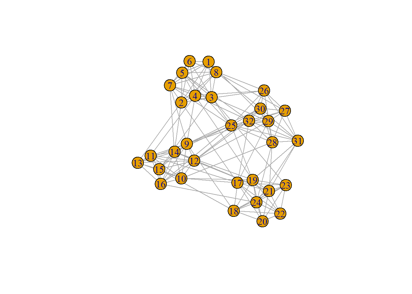
Perhaps you are randomly placed onto subject 1. From subject 1, you decide to “take a walk” through the network. We might ask:
“What is the probability that you will go from subject 1 to any other subject in a walk of length \(s\)?”
What you’ll find is that–generally–walks throughout a network will generally end up with subjects being “trapped” within certain communities. Logically, this should make sense. When you walk down your neighborhood, you don’t often randomly end up in Los Angeles [unless you live there]. You could end up there but it’s certainly not more likely than you remaining in your neighborhood.
Now for the formalism.
WalkTrap operates by recasting our adjacency matrix, \(\mathbf{A}\), into a probability transition matrix given by:
\[\mathbf{P} = \mathbf{D}^{-1}\mathbf{A}\] where \(\mathbf{D}\) is a diagonal matrix that contains the degree [or strength] of each node on its diagonal. Essentially, what this does is it divides our values in our adjacency matrix by the degree/strength of each node and turns them into probabilites of moving from one node to another.
For example, in a binary graph, I might have a degree of 5 which means that I have 5-connections to other individuals. The corresponding probability that I move from myself to any of my other 5-connections is then \(\frac{1}{5}\). The expression above is just the matrix way of doing that in one pass!
Great. So, now we have \(\mathbf{P}\). Now what? Recall in the first week when I discussed the “powers of the adjacency matrix”. In that lesson, we discussed how exponentiating an adjacency matrix gives you the distance in however many exponentiated steps.
So then:
\[\mathbf{P}^{4}\] would tell me the probability of moving from any given person to any other person in \(4\) steps. We can then use these distances to generate some distances as:
\[r^{2}_{ij} = \sum_{k}\frac{1}{d_{k}}\left( p_{ik}^{t} - p_{jk}^{t} \right)^{2}\] here, \(r^{2}_{ij}\) is the squared distance between subjects \(i\) and \(j\) which depends on:
- \(d_{k}\): the degree of the \(k^{th}\) subject
- \(p_{ik}^{t}\): the probability of going from subject \(i\) to subject \(k\) in \(t\) steps
- \(p_{jk}^{t}\): the probability of going from subject \(j\) to subject \(k\) in \(t\) steps
for all of \(k\) subjects. That is, the distance between 2-subjects is smaller if they tend to reach the same other subjects in the same number of steps. By contrast, if a subject is highly unlikely to reach the same subjects are you then we’d say you’re probability “far” from one another.
Well, that’s great. We have turned our data into a new, fancy matrix but we need to find an objective function to optimze on or else it’s not all that helpful, is it?
Next up, we discuss the objective function of WalkTrap: modularity (or \(Q\))
Modularity, \(Q\)
Modularity has a unique definition that is quite intuitive:
\[Q = \frac{1}{2m}\sum_{ij}\left[ a_{ij} - \frac{d_{i} d_{j}}{2m} \right]\delta(c_{i},c_{j})\] where \(Q\) is a value that represents the difference between the observed similarity between subjects \(i\) and \(j\) compared to the product of their degrees divided by \(2m\)–the total number of possible edges in an undirected graph if we assume that both directions are counted.
Put another way, \(Q\) represents the difference between what we observed \(a_{ij}\) and what we expected by chance \(\frac{d_{i} d_{j}}{2m}\). Thus, if we optimize on modularity, we should obtain a cluster solution whose subgroups are more connected to one another than they would be expected to by random chance.
So, how do we actually run WalkTrap?
- Initialize using a method called, “Ward’s Criterion”
- This approach places everyone in a single group comprised of just them
- Next, it looks at merging every pair of subjects
- Any merge will make the fit of the model worse
- Select the merge that would worsen fit the least
- Repeat this iteratively until all individuals are in a single group
- Identify the “partition” related to when \(Q\) was highest
In \(\texttt{R}\) we can do this by:
ng = graph_from_adjacency_matrix(adjacency.matrix,
                                 mode = "undirected",
                                 diag = FALSE,
                                 weighted = TRUE)
plot(ng)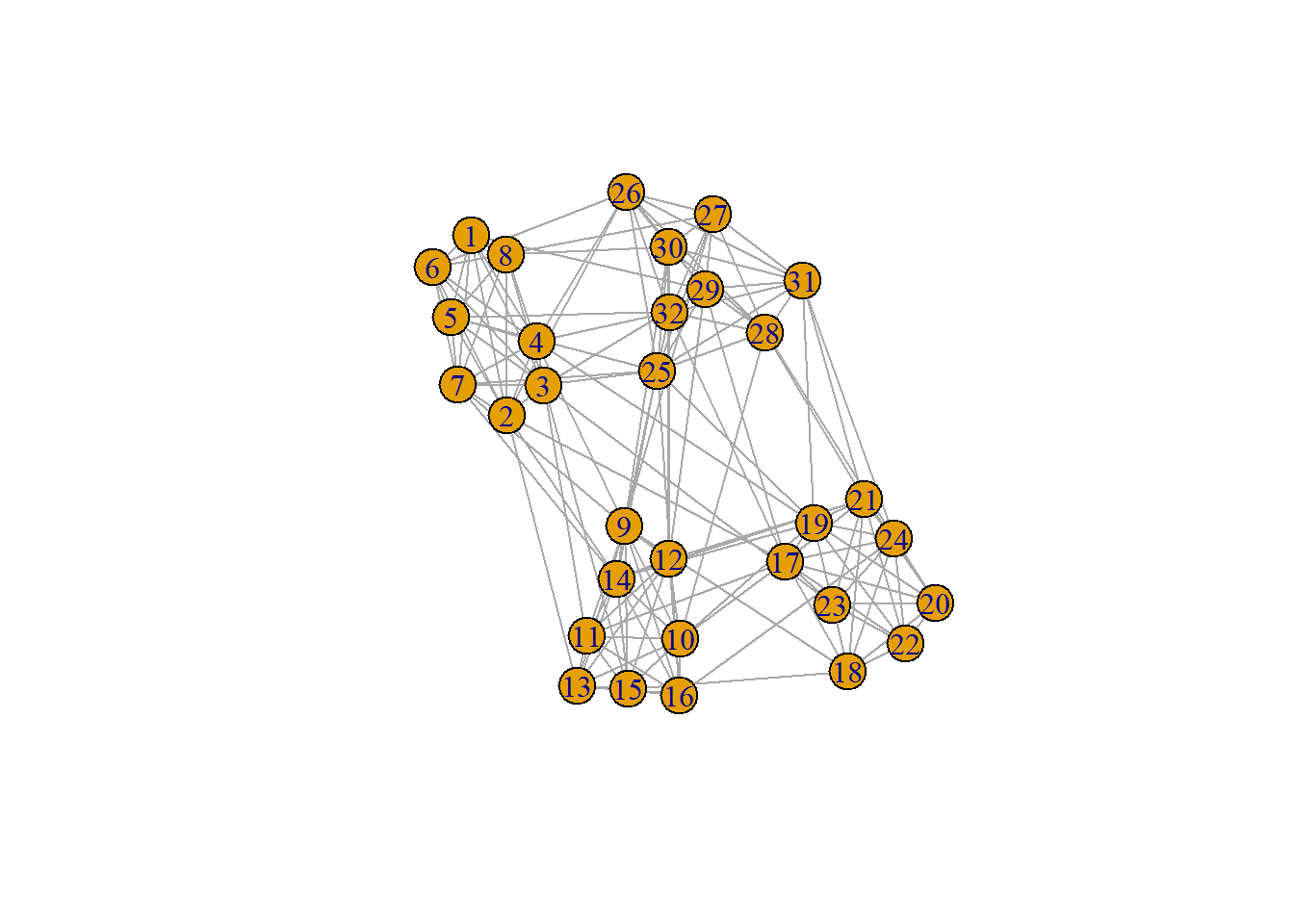
groups = cluster_walktrap(ng)
plot(groups, ng)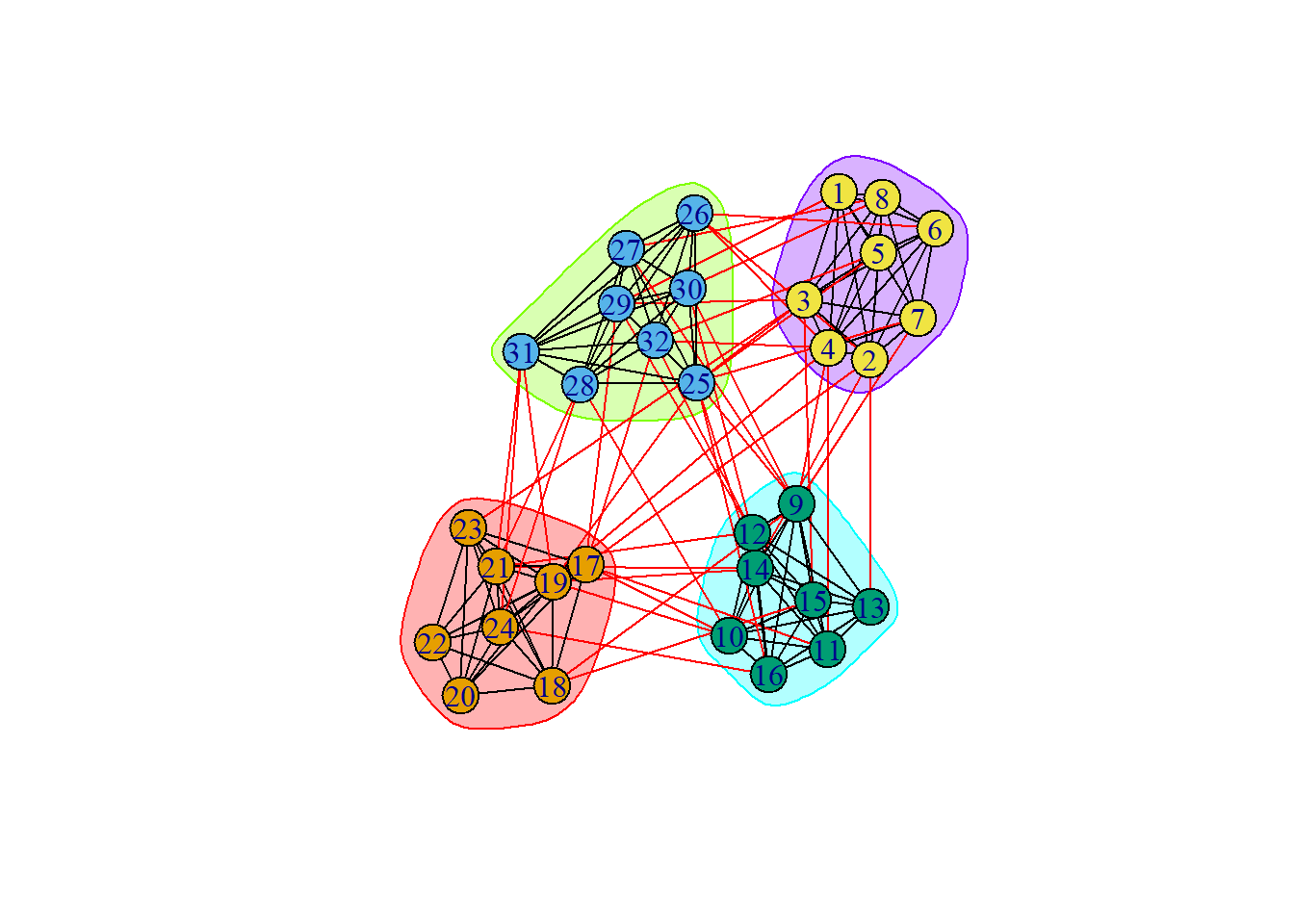
First, we turned our adjacency matrix into a graph that \(\texttt{igraph}\) can recognize. Then, we plotted the empty graph.
Then, we create an object called, “\(\texttt{groups}\)” which contains the WalkTrap solutions and then we can plot the groups we recovered.
We may also choose to extract the raw group memberships like we did with fuzzy \(c\)-means and \(k\)-means:
groups$membership [1] 4 4 4 4 4 4 4 4 3 3 3 3 3 3 3 3 1 1 1 1 1 1 1 1 2 2 2 2 2 2 2 2We can also view our modularity value:
round(modularity(groups), 3)[1] 0.594In this case, our modularity is nearly \(0.60\). If it were close to \(0.00\) that could be concerning but it’s indicating that–generally–our clusters tend to have more within-community connections than we would expect by chance. So, that’s decent.
In some of the papers this week, you may have seen that WalkTrap could be improved upon by simply integrating a different method than Ward’s Criterion.
Let’s talk a bit about why that was the case.
Answer.
Ward’s Criterion is what is referred to as a hierarchical agglomerative clustering algorithm. What this means is that it forms clusters as a hierarchy. Starting from everyone as a cluster on their own and slowly conducting merges at each step.
The issue that arises with this is that if you make a mistake in a merge, you cannot change your mind. By contrast, \(k\)-means is always shuffling people back and forth to identify its centroids. This is computationally more expensive but may prevent \(k\)-means from getting trapped like Ward’s Criterion.
Assessing Cluster Quality
Okay, so now we have our cluster solutions. In the real-world, we cannot always know what the true group memberships are; however, in this example we actually do and thanks to that, we can assess the accuracy of our methods:
results = data.frame(k.Means = results.1[[n.groups]]$cluster,
                     c.Means = results.2[[n.groups]]$cluster,
                     WalkTrap = groups$membership,
                     True = rep(1:n.groups, each = n.nodes.per.group))
ARIs = data.frame(k.Means = adjustedRandIndex(results$k.Means, results$True),
                  c.Means = adjustedRandIndex(results$c.Means, results$True),
                  WalkTrap = adjustedRandIndex(results$WalkTrap, results$True))

ARIs
k.Means c.Means WalkTrap
1 1 1 1From this output, we can see that \(k\)-means, fuzzy \(c\)-means, and WalkTrap all received an ARI score of \(1.00\). But, what is the ARI?
ARI stands for the Adjusted Rand Index and it takes on values ranging from \(0.00\) to \(1.00\) where \(0.00\) indicates chance performance and \(1.00\) indicates perfect performance or classification. Generally, values at or above \(0.90\) would be considered excellent classification.
Concluding Remarks
Ultimately, these community detection approaches are a means of studying the interrelations among our data and finding “partitions”, “clusters”, “communities”, “subgroups” of variables that tend to belong with one another. The methods we covered today: \(k\)-means, fuzzy \(c\)-means, and WalkTrap are all approaches for identifying communities that have their own strengths and limitations.
Let’s recap.
\(k\)-means
\(k\)-means has a long history of application in many, many fields. It’s incredibly robust and relatively simple to implement. In our example, it found the correct number of communities and assigned people to the correct groups.
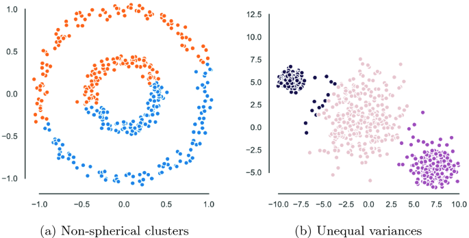
However, it also has known limitations. For example, \(k\)-means–without modifications–only extracts “spherical” clusters. What this means is that the communities identified by \(k\)-means will always be circles around the “centroids”. Sometimes, communities are not perfectly organized. For example, in the image below [left panel], \(k\)-means would fail to find that there are 2-communities: the inner and outer community.
This is because \(k\)-means cannot deal with complex or “bending” clusters.
Fuzzy \(c\)-means
This limitation is shared by fuzzy \(c\)-means when not adapted to model covariances in the cluster solutions; however, \(c\)-means has an advantage over \(k\)-means in that it adds a component of ambiguity to our analysis and allows us to observe not only if people belong in communities but if we are confident in their assignments.
Ultimately, both \(k\)-means and \(c\)-means are limited in that they need some predetermined number of communities to be selected. If we don’t have prior theory, this can be difficult because we can only use statistical comparisons. If we do this in an ethical way and discuss that our analyses are exploratory, that is fine.
WalkTrap
By contrast, WalkTrap with Modularity maximization can find community structures by optimizing for the best Modularity value. Thus, it does not need a pre-specified number of communities and is fully exploratory. However, this leads to a question as to whether Modularity is a good function to optimize on.
Logically, it makes sense that expecting two nodes to be more connected than we would–on average–expect is appealing; however, some readings this week cautioned on limitations of Modularity maximization.
Likewise, unlike fuzzy \(c\)-means, WalkTrap doesn’t model ambiguity in cluster assignments explicitly. We know our real-world systems are likely not truly hard group structures. So, how do we reconcile these different approaches?
Is there one best model or approach?