# Installing or calling packages
# install.packages('multinet')
library(multinet)
library(igraph)
library(poweRlaw)
library(Matrix)


net <- read_ml("example_multiplex.mpx")PSC-290: Multilayer and Multiplex Networks
Review Simple Undirected Graphs
A simple undirected graph is the foundational concept in network science used to represent complex systems characterized by interacting units. In its most basic form, a network reduces a system to an abstract structure consisting of entities called nodes (or vertices) and the connection patterns between them, called edges.
In an undirected graph, the set of edges is unordered, meaning a connection between node i and node j is the same as a connection between node j and node i. The term “simple” often implies that edges are unweighted (binary, representing presence or absence of a connection) and that there are no self-loops (edges connecting a node to itself) or multiple edges between the same pair of nodes.
Simple undirected graphs allow for the quantification and description of network structure and dynamics using various measures:
Node-level:
The degree of a node is the number of edges it possesses. In weighted networks, this is extended to strength.
Centrality measures quantify a node’s importance, such as degree centrality (nodes with more edges affecting a larger group), eigenvector centrality (importance based on being linked to other important nodes), and betweenness centrality (fraction of shortest paths between other nodes that pass through a given node).
The clustering coefficient of a node measures the interconnectedness of its neighbors.
Group-level:
- Transitivity or the global clustering coefficient is the fraction of paths of length three in the network that are closed, quantifying the level of transitivity in the network.
- Community detection identifies groups or modules of nodes that are more densely connected among themselves than to nodes outside the group, often based on maximizing network modularity.
Network-level:
- The degree distribution describes the fraction of nodes with a given degree.
- Distance measures, such as the shortest path length between nodes and the diameter (maximum distance between any two nodes), characterize the metric structure. Language networks, for instance, often show small-world properties, characterized by relatively short characteristic path length and high clustering.
Extend to Temporal Networks
Temporal networks are a type of network structure that explicitly addresses the time-varying nature of interactions. They represent systems where the connections between nodes evolve over time. The multilayer network framework provides a natural and powerful way to represent these temporal dynamics.
In a multilayer network representation of a temporal network, each distinct point or window in time can be modeled as a separate layer. This means if you observe the network at different time steps or over consecutive periods, each time slice becomes one layer in the multilayer structure.
The nodes typically persist across these time layers. For instance, in a social network observed daily, the individuals remain the same, but their interactions (edges) might change from one day’s layer to the next. The intralayer edges within each time layer represent the interactions occurring during that specific time period. These intralayer edges can be weighted or unweighted, directed or undirected, depending on the nature of the interactions at that time.
Interlayer edges connect these temporal layers. In the case of temporal networks, these interlayer edges often connect a node in one time layer to its corresponding “copy” or “node-tuple” in an adjacent time layer. These connections explicitly encode the temporal link or persistence of the node from one time point to the next. These layers are typically ordered sequentially in time (ordinal coupling).
Make the leap from Temporal to Multiplex Networks
What are Multiplexes?
Multiplex networks are presented as a special type of multilayer network. They are characterized by having the exact same set of nodes present in every layer. These identical nodes across layers are referred to as “replica nodes” or “node-tuples”.
The layers in a multiplex network represent different types of interactions or relationships that exist simultaneously or in parallel between the same set of nodes. For example, in a social system, one layer might represent friendships, another professional connections, and another family ties, all involving the same individuals (nodes). In ecological systems, layers could represent different interaction types like trophic (predator-prey) and non-trophic (e.g., facilitation) relationships between the same species. In biological systems, layers could be different molecular interaction networks (e.g., protein-protein, gene regulation). In transportation, layers could be different modes like road, rail, or air between the same locations.
A defining feature of multiplex networks, in their strict definition, is that the interlayer connections (or couplings) exist only between a node and its corresponding replica node in other layers. This means node ‘A’ in layer 1 can only be connected to node ‘A’ in layer 2, node ‘A’ in layer 3, and so on, but not to node ‘B’ in any other layer.
Multiplex networks allow researchers to study how different types of relationships between the same nodes interact and influence system properties. They can reveal insights into node importance across different contexts (versatility), the overlap of connections across layers, and how dynamics like spreading or synchronization are affected by the presence of multiple interaction types.
How do they differ from Temporal Networks as we learned them?
The key differences lie in what the layers represent and the pattern of interlayer connections:
Meaning of Layers: In the multilayer representation of a Temporal Network, layers represent different points or windows in time. In a Multiplex Network, layers represent different types of relationships or interaction categories between the same nodes.
Interlayer Connection Pattern:
Temporal Networks typically employ ordinal coupling, connecting a node’s replica in one time layer only to its replica in the immediately preceding and succeeding time layers.
Multiplex Networks have interlayer connections between a node’s replica in any layer and its replica in every other layer where it exists (all-to-all replica coupling).
Both Temporal and Multiplex networks are specific types of Multilayer Networks. Temporal networks use the multilayer structure to model the evolution of connections over time, while Multiplex networks use it to model the coexistence of different types of relationships over the same set of nodes.
Extend to Multilayer Networks
Multilayer networks are a more general framework developed to account for systems where different networks interact or evolve with each other. In a multilayer framework, a system is represented by structures that have layers in addition to nodes and edges. Layers represent aspects or features that characterize the nodes or edges belonging to that layer. The set of edges is partitioned into intralayer edges (connecting nodes within the same layer) and interlayer or coupling edges (connecting nodes in different layers). In its most general form, a node in layer α can be connected to any node in any layer β.
A multilayer network can be formally defined as a pair M = (G, C) where G = {Gα; α ∈ {1, . . . ,M}} is a family of graphs (layers), and C = {Eαβ ⊆ Xα × Xβ; α, β ∈ {1, . . . ,M}, α ≠ β} is the set of interconnections between nodes of different layers. Here, Gα = (Xα, Eα) represents the graph of layer α, with Xα being the set of nodes and Eα the set of edges in that layer.
Multiplex Networks are presented as a special type of multilayer network.
- Interlayer Coupling: the interlayer connections (coupling edges) exist only between a node and its corresponding counterpart node (replica) in the rest of the layers. In a general Multilayer Network, interlayer connections are not restricted to connecting only replica nodes; a node in one layer can potentially connect to any node in another layer.
We will use the following network data through out this session. The nodes in this network are the typical symptoms of psychopathology, and the layers are different aspects of psychopathology, namely, temporal, neural, genetic, behavioral, and clinical cluster. The network serves to model how symptoms are connected under each of the aspects.
To begin with, install/call the following packages:
If you want to use your own network data, run net = your network data; otherwise, we can take a glimpse of the current network’s structure:
# Setting up and Transforming datasets
# net = your network data
# We see the density, clustering coefficient, average path length, diameter
summary(net)
n m dir nc slc dens cc apl dia
_flat_ 33 522 0 1 33 0.9886364 0.6508500 1.577652 3
behavioral 18 21 0 1 18 0.1372549 0.2790698 3.797386 10
clinical_cluster 29 82 0 1 29 0.2019704 0.4125000 2.270936 5
genetic 32 161 0 1 32 0.3245968 0.5454545 1.770161 3
neural 24 106 0 1 24 0.3840580 0.5623160 1.681159 3
temporal 33 152 0 1 33 0.2878788 0.4991394 1.831439 3Here, n is the number of verticies, m is the number of edges, dir is the directionality (undirected/directed), nc is the number of components (strongly connected components for directed graphs), slc is the size of largest (strongly connected) component, dens is the density , cc is the clustering coefficient, apl is the average path length, and d is the diameter.
As you can see, not every node (symptom) presents on each of the layers.
You can also plot each layer’s network:
plot(net, layers = 'temporal')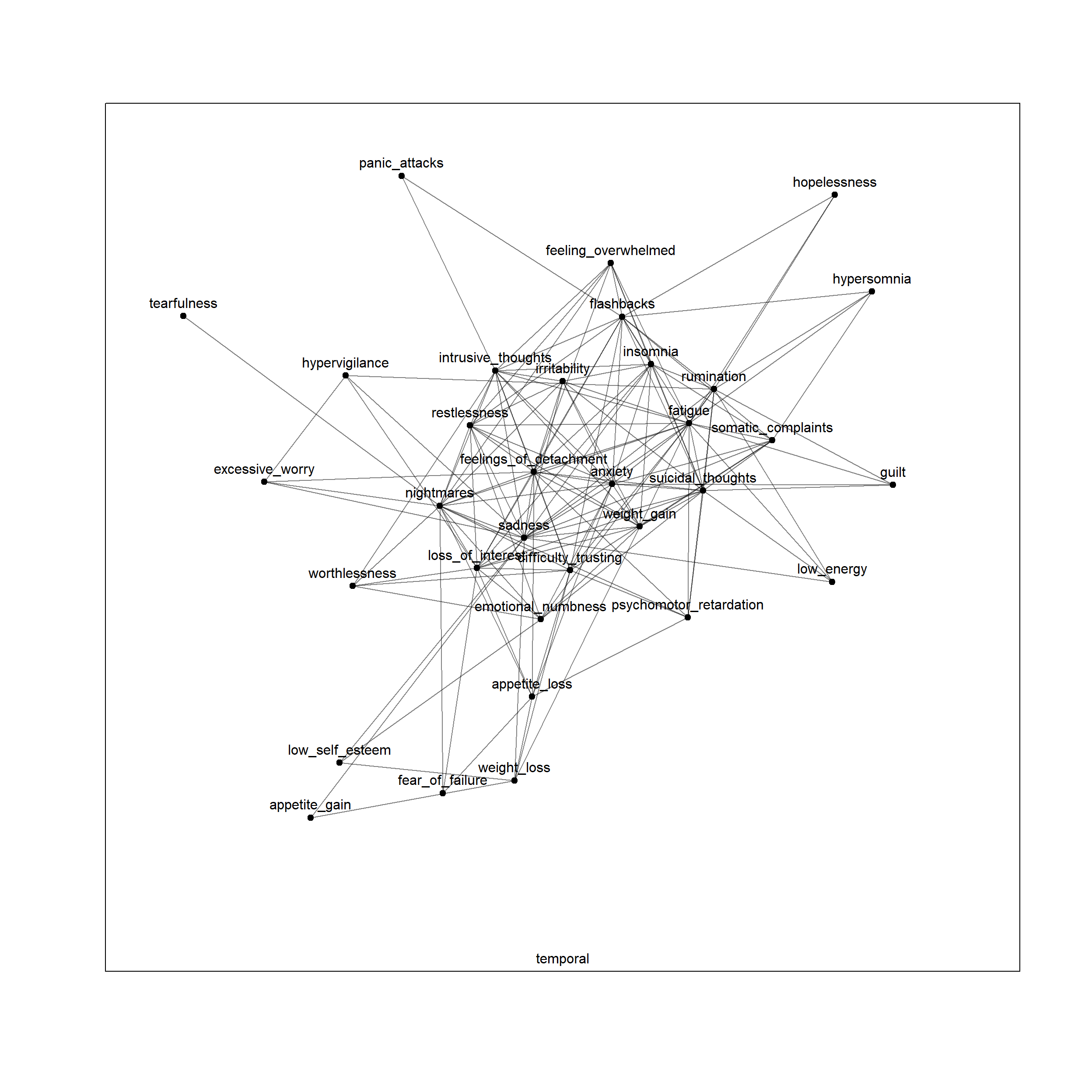
plot(net, layers = 'neural')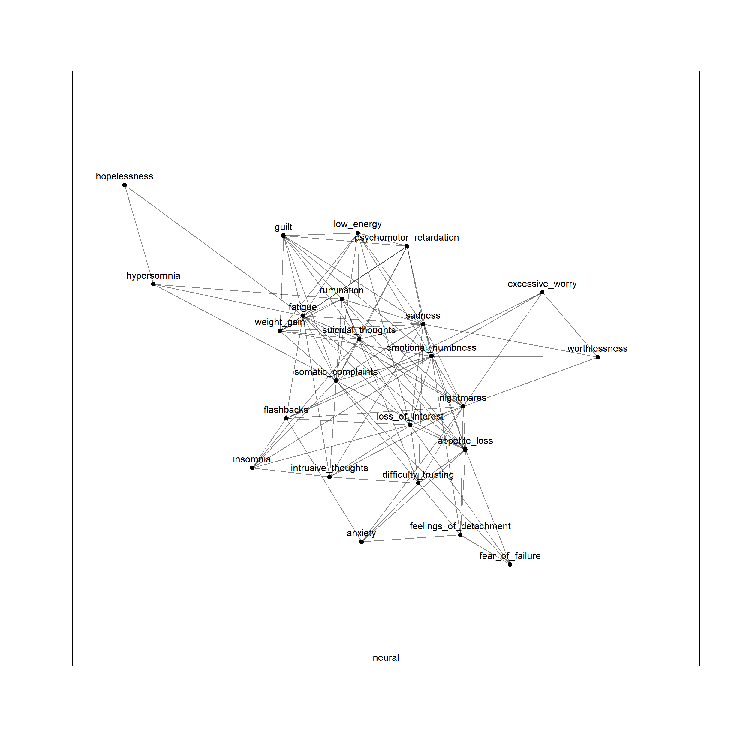
plot(net, layers = 'behavioral')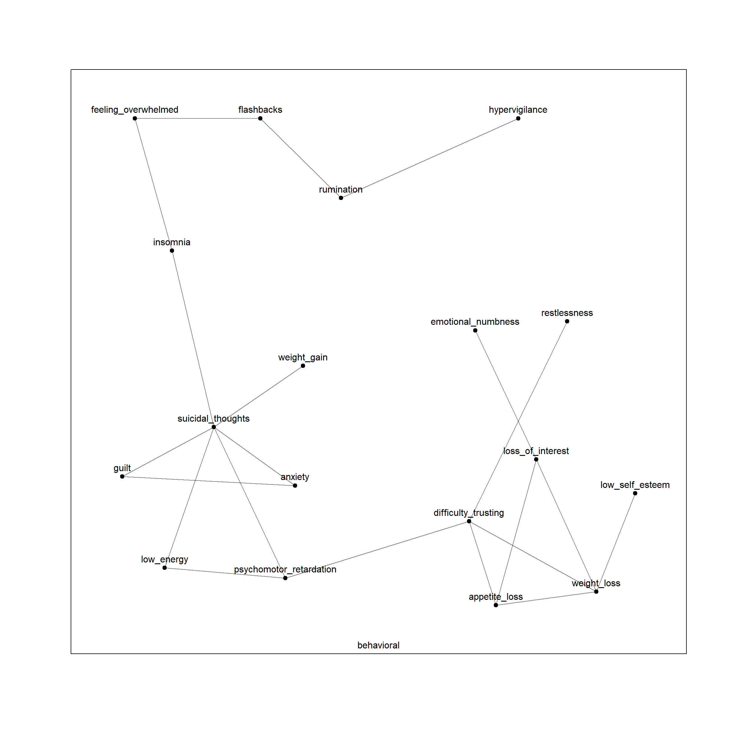
plot(net, layers = 'genetic')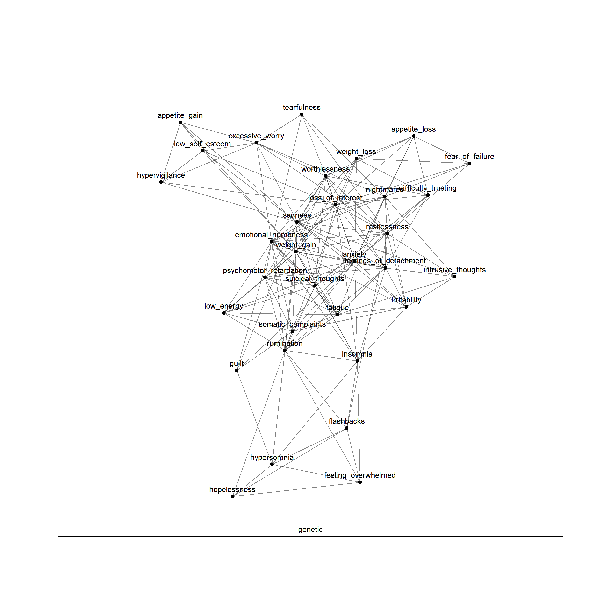
plot(net, layers = 'clinical_cluster')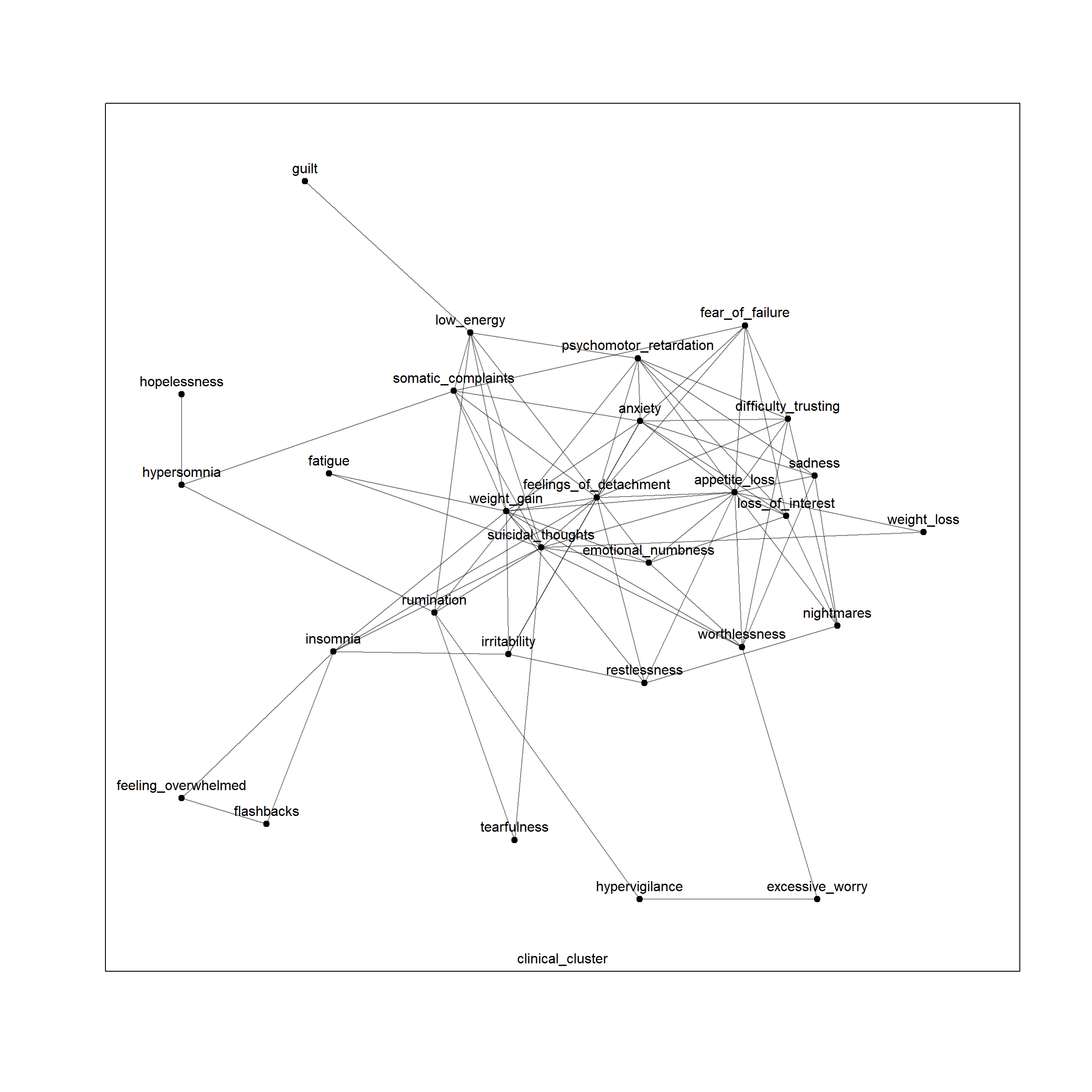
Question: Is this network multiplex or multilayer?
This is a multiplex network, since interlayer connections only exist between corresponding nodes across layers.
Recast a Multilayer and/or Multiplex Network as an Undirected Simple Graph
It is possible to represent both multiplex and more general multilayer networks as a single, larger graph, often referred to as a flattened network, aggregated network, or a “flatiplex” graph constructed from the “disjoint union” of all the nodes from all layers.
The following function can be used to transform a multiplex network to and from a flatiplex network:
# Flat graph and back:
to.and.fro = function(input = NULL, goal = c("flat", "multiplex")) {
  # Define our goal:
  goal = match.arg(goal)
  # Code for turning multiplex into a flatiplex [lol]
  if (goal == "flat") {
    if (!inherits(input, "Rcpp_RMLNetwork")) {
      stop("Input must be a multinet object when goal is 'Flat'")
    }
    # Extract layer names and make empty list
    layer.names = layers_ml(input)
    all.edges = list()
    # For each layer, see who is connected to whom
    # Create super list of all people who are connected in each layer
    for (layer in layer.names) {
      edges = edges_ml(input, layer)
      edges = data.frame(from = edges$from_actor,
                         to = edges$to_actor,
                         layer = layer,
                         stringsAsFactors = FALSE)
      all.edges[[layer]] = edges
    }
    df = do.call(rbind, all.edges)
    # Connect individuals in alphabetical order
    df$pair = ifelse(df$from < df$to,
                     paste(df$from, df$to, sep = "--"),
                     paste(df$to, df$from, sep = "--"))
    # Dummy code the variables and split names into different columns
    # Remove the row names to clean up
    temp.mat = with(df, table(pair, layer))
    split.pairs = strsplit(rownames(temp.mat), "--")
    pair.df = as.data.frame(do.call(rbind, split.pairs),
                            stringsAsFactors = FALSE)
    colnames(pair.df) = c("from", "to")
    the.graph = cbind(pair.df, as.data.frame.matrix(temp.mat))
    rownames(the.graph) = NULL
    return(the.graph)
  }
  # Code for flatiplex to multiplex
  if (goal == "multiplex") {
    if (!is.data.frame(input)) {
      stop("Input must be a data.frame when goal is 'Multiplex'")
    }
    required_cols = c("from", "to")
    if (!all(required_cols %in% names(input))) {
      stop("Input must contain 'from' and 'to' columns")
    }
    # Create an empty multilayer network with the predefined layer names
    col.layers = as.character(setdiff(names(input), required_cols))
    net = ml_empty()
    add_layers_ml(net, col.layers)
    # Find who exists in which layer
    # Populate the graphs
    vertex.pairs = unique(do.call(rbind, lapply(col.layers,
                                                function(layer) {
      rows = which(input[[layer]] == 1)
      actors = unique(c(input$from[rows], input$to[rows]))
      data.frame(actor = actors, layer = layer, stringsAsFactors = FALSE)
    })))
    add_vertices_ml(net, vertex.pairs)
    # At connections for people within each layer if they were connected in
      # The flatiplex network
    for (layer in col.layers) {
      present = input[[layer]] == 1
      if (any(present)) {
        edges = input[present, c("from", "to")]
        edges = data.frame(edges$from, layer, edges$to, layer,
                           stringsAsFactors = FALSE)
        add_edges_ml(net, edges)
      }
    }
    return(net)
  }
}
We first transform our multiplex network to a flatiplex network:
# Test movement between graphs:
flat = to.and.fro(net, goal = "flat")
head(flat)
from to behavioral clinical_cluster genetic neural
1 anxiety appetite_loss 0 1 1 1
2 anxiety difficulty_trusting 0 1 1 1
3 anxiety emotional_numbness 0 0 1 0
4 anxiety fatigue 0 0 0 0
5 anxiety fear_of_failure 0 1 1 0
6 anxiety feelings_of_detachment 0 1 1 1
temporal
1 1
2 1
3 1
4 1
5 0
6 1Each row in this data frame represent edges between two nodes. For example, the first row is the edges between anxiety and appetite_loss. If a edge between two nodes exist on a layer, the layer gets a 1; otherwise, the layer value is 0. Therefore, the anxiety-appetite_loss edges are 1 on the clinical_cluster, genetics, neural, and temporal layers, but not on the behavioral layer.
We can also count the number of total edges two nodes have, and save them as the weights:
# Condense the flatiplex network using weights, i.e., how many edges between two nodes in total accross layers, based on the dataframe above
flat$weight = rowSums(flat[ , 3:ncol(flat)])
Then we plot the nodes with the weights > 0 (i.e., when there is a least one edge between two nodes):
theflatjack = graph_from_data_frame(flat[flat$weight > 0,
                                           c("from", "to", "weight")],
                                      directed = FALSE)
plot(theflatjack)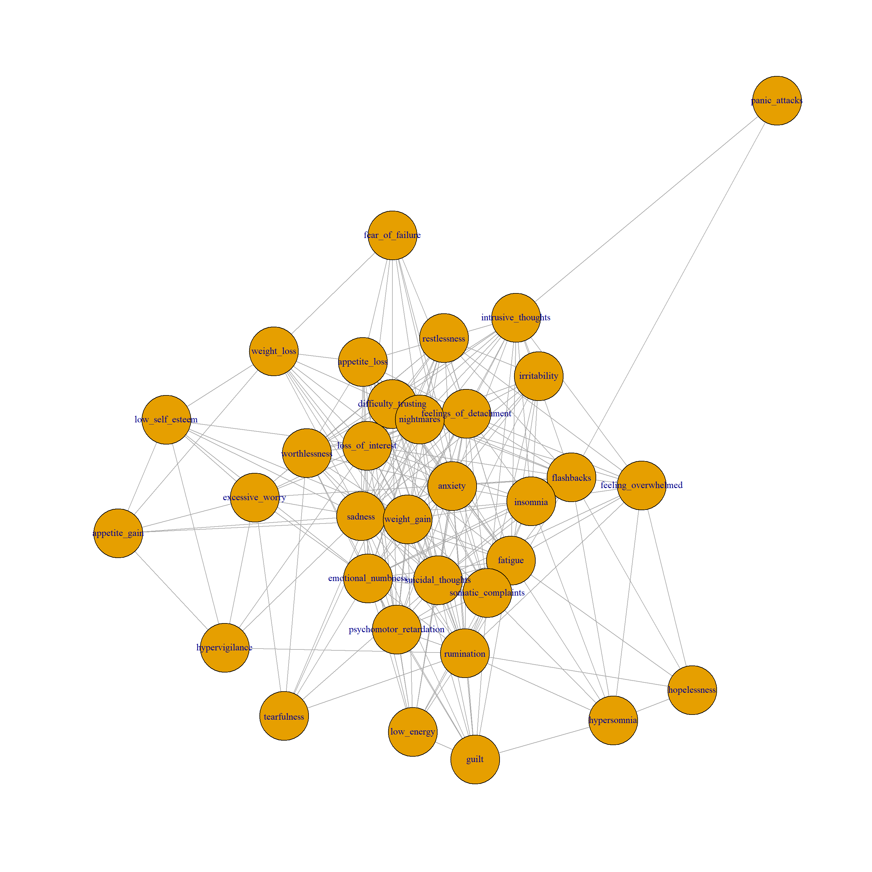
Does the flatjack network maintain the original multiplex network’s density?
edge_density(theflatjack)[1] 0.4583333summary(net)$dens[1][1] 0.9886364Doesn’t seem so. What about the mean of each layer’s densities?
mean(summary(net)$dens[2:6])[1] 0.2671518Nope. So, why is that?
We now transform our flatiplex network back to multiplex:
# Finally, we can move back to the multiplex:
multi = to.and.fro(flat, "multiplex")
summary(multi)
n m dir nc slc dens cc apl dia
_flat_ 33 604 0 1 33 1.1439394 0.6508500 1.577652 3
behavioral 18 21 0 1 18 0.1372549 0.2790698 3.797386 10
clinical_cluster 29 82 0 1 29 0.2019704 0.4125000 2.270936 5
genetic 32 161 0 1 32 0.3245968 0.5454545 1.770161 3
neural 24 106 0 1 24 0.3840580 0.5623160 1.681159 3
temporal 33 152 0 1 33 0.2878788 0.4991394 1.831439 3
weight 33 82 0 1 33 0.1553030 0.1598063 2.357955 5summary(net) n m dir nc slc dens cc apl dia
_flat_ 33 522 0 1 33 0.9886364 0.6508500 1.577652 3
behavioral 18 21 0 1 18 0.1372549 0.2790698 3.797386 10
clinical_cluster 29 82 0 1 29 0.2019704 0.4125000 2.270936 5
genetic 32 161 0 1 32 0.3245968 0.5454545 1.770161 3
neural 24 106 0 1 24 0.3840580 0.5623160 1.681159 3
temporal 33 152 0 1 33 0.2878788 0.4991394 1.831439 3What Information is Lost via Compression and Why We Would Not Want to Do This
Compressing a multilayer or multiplex network into a single, flattened graph results in a loss of information about the original system’s structure and context. This is why the traditional single-layer approach is often insufficient for complex systems.
Here’s what is lost and why we wouldn’t want to do this:
The Meaning and Identity of Layers: When you flatten a multilayer network, the explicit distinction between different types of interactions (e.g., shared genetic cause vs. shared behavioral cause) represented by the original layers is lost. The resulting single graph does not indicate the original layer or relationship type these links belonged to.
The Nature of Interlayer Connections: The specific patterns of interlayer connections, which encode crucial relationships between layers (like persistence through time, or dependence across interaction types), are collapsed into simple edges in the flattened graph. This loses information about which layers are connected and how they are connected (e.g., is it a replica connection, a connection to a different node, is it weighted?).
Distinct Properties and Dynamics: Many properties and dynamical processes manifest differently on multilayer/multiplex networks compared to their aggregated single-layer counterparts. By compressing, you lose the ability to accurately study these layer-dependent or interlayer-influenced phenomena.
Boccaletti et al., 2014provides numerous examples:Network Structure and Metrics: Measures like degree become vectors in multilayer networks, not scalars. Aggregating loses this vectorial nature, forcing the use of aggregated measures like “overlapping degree”, which conflate distinct information. Concepts like “edge overlap” which count how many layers a specific link appears in are specific to multilayer structures and lost in single-layer views, unless the single-layer view explicitly preserves this count as edge weight. Other measures like multi-triads and multilayer clustering coefficients capture structural patterns that span layers, which are not visible in aggregated networks.
Robustness and Percolation: Studies show that interdependent networks (a type of multilayer) exhibit catastrophic cascading failures and discontinuous percolation transitions, unlike the continuous transitions often seen in single-layer networks. Compressing would obscure this critical difference in robustness. For multiplex networks specifically, robustness under random node removal shows a hybrid transition. This behavior is fundamentally tied to the multilayer structure.
Diffusion and Spreading: Diffusion processes like random walks or epidemic spreading on multilayer networks can behave differently, exhibiting faster diffusion or modified epidemic thresholds, compared to isolated or aggregated layers. Aggregating into a single layer would lead to incorrect predictions about how things spread or flow. For example,
Boccaletti et al., 2014explicitly discusses how simulating a classical diffusion model on a single-layer Facebook network (ignoring different friendship types) would lead to “incorrect conclusions and predictions of the real dynamics”.
Boccaletti et al., 2014 offers illustrative examples of why single-layer models fail:
Social Networks: Facebook friendships arising from different origins (colleagues, fans, etc.) have different implications for information spreading. Representing Facebook as a single network of acquaintances, as in the traditional approach, and simulating a classical diffusion model would give incorrect predictions because the dynamics depend on the type of relationship, not just its existence.
Transportation Networks: The Air Transportation Network (ATN) involves different airlines, each forming a distinct layer. Simulating delay propagation or passenger rescheduling by representing the ATN as a single-layer network (as traditionally done) leads to incorrect conclusions. Rescheduling costs and priorities depend on whether a passenger is moved within the same airline’s network or to another company’s network, a detail lost in a single aggregated layer.
Therefore, while a supra-adjacency matrix provides a mathematical representation, collapsing a multilayer or multiplex network into a simple graph loses the very information about context, relationship types, and interlayer dependencies that makes the multilayer framework powerful for understanding complex systems.
When is it okay to aggregate (flatten) a multilayer network?
De Domenico et al. (2015a) tackle the problem of reducibility, i.e., defining the number of layers a multilayer network needs to have to accurately represent the structure of the system. Using the Von Neumann entropy on a multilayer network it is possible to determine if the multilayer representation is distinguishable from the aggregated network. This way, they propose that if the aggregation of two layers does not result in a decrease of the relative entropy with respect to the multiplex where they are separated, they should be kept aggregated. (Aleta & Moreno, 2018)
Framing a Temporal Network as both a Multiplex and as a Multilayer
Temporal networks can be naturally represented using multilayer networks.
In this representation:
Each layer corresponds to a distinct point or window in time when interactions are observed.
The entities (nodes) typically persist across these time layers.
Intralayer edges within a layer represent interactions occurring during that specific time period.
Interlayer edges connect a node in one time layer to its corresponding replica in a different time layer.
This structure fits the general definition of a multilayer Network because it uses layers to represent distinct aspects (time points) and includes both intralayer and interlayer connections.
Now, let’s consider if a temporal network, framed this way, is also a multiplex Network. Based on the strict definition of a multiplex network:
It must have the exact same set of nodes in every layer. Temporal network representations often assume a fixed set of possible nodes across time steps, even if some are inactive, which aligns with this.
The only permissible interlayer connections are between a node and its counterpart (replica) in the rest of the layers. Temporal networks, when represented as multilayer structures, typically feature interlayer connections between a node in one time layer and its replica only in the immediately preceding and succeeding time layers. This is referred to as ordinal coupling.
So, while temporal networks satisfy the first condition (same node set across layers, or at least a consistent potential set), they often violate the second condition by restricting interlayer coupling to adjacent layers (ordinal coupling) rather than allowing connections between replica nodes across all layers (all-to-all replica coupling).
Therefore, a temporal network represented as a multilayer structure is a type of multilayer metwork, specifically one where layers are ordered in time and interlayer coupling is typically ordinal. It is similar to a multiplex network in that it has the same set of nodes across layers and uses replica-to-replica interlayer coupling, but the pattern of interlayer coupling (ordinal vs. all-to-all) distinguishes it from the strict definition of a multiplex Network. However, the term “multiplex” is sometimes used more broadly in the literature to encompass any multilayer network with the same set of nodes, regardless of the interlayer coupling pattern. It’s more accurate to describe it as a specific type of multilayer network with temporal layers and ordinal coupling, which shares characteristics with multiplex networks (node set, replica coupling) but differs in the coupling pattern.
Centrality/Node Importance in Multilayer Networks
Degree
In a single-layer network, the degree of a node is a basic measure of its importance, defined as the number of links it possesses. Nodes with many links (high degree) can influence a large number of other nodes. The degree of node \(i\) is calculated by summing the entries of the adjacency matrix A, where $( a_{ij} $) = 1 if a link exists between \(i\) and \(j\) (or a weight w for weighted networks) and 0 otherwise: \(k_i = \sum_{j=1}^{N} a_{ij}\). The degree distribution, pk (fraction of nodes with degree \(k\)), characterizes the network structure.
Extending this to a multilayer network, a node’s degree is no longer a single scalar value but is represented as a vector, known as the multidegree. For a multiplex network with L layers, the degree of node i is the vector ki = {k1i, …, kLi}, where kαi is the degree of node i in layer α. The degree kαi is calculated by summing the entries of the adjacency matrix for layer α, Aα: $k_{i} = {j} a_{ij} $.
The logic of this transformation is that a node’s connectivity can vary significantly across different types of interactions or layers. Representing the degree as a vector captures this layer-specific importance, providing a more detailed view than a single number. To obtain a single value for ranking nodes across the entire multilayer network, aggregated measures can be used, such as the total degree or degree overlap, which is the sum of degrees across all layers: \(o_i = \sum_{\alpha} k_{\alpha i}\).
(fl.deg = degree(theflatjack)) anxiety appetite_gain appetite_loss
23 6 17
difficulty_trusting emotional_numbness excessive_worry
17 21 11
fatigue fear_of_failure feeling_overwhelmed
22 8 11
feelings_of_detachment flashbacks guilt
22 18 11
hopelessness hypersomnia hypervigilance
5 8 6
insomnia intrusive_thoughts irritability
14 16 11
loss_of_interest low_energy low_self_esteem
21 11 8
nightmares psychomotor_retardation restlessness
20 16 17
rumination sadness somatic_complaints
22 25 19
suicidal_thoughts tearfulness weight_gain
22 7 21
weight_loss worthlessness panic_attacks
11 15 2 Single-layer and multilayer degree metrics can disagree. Calculating centrality measures in the context of multilayer networks makes it possible to find versatile nodes which cannot be directly extracted from the aggregated network. For example, in a study of baboon social networks represented as a two-layer multiplex (grooming and association), the most central individual in the multilayer representation was not highly central in the aggregated single-layer network or in the individual layers (Finn et al., 2017). This demonstrates that simply summing or averaging degrees across layers (aggregation) does not capture the same information as a multilayer analysis, and nodes important across multiple interaction types or layers may be missed in a single-layer view.
ml.deg = NULL
# Use a for loop to maintain same node order between mutliplex and flatiplex
for(symptom in names(fl.deg)){
      ml.deg = c(ml.deg, degree_ml(net, actors = symptom))
}
ml.deg
[1] 52 7 44 39 47 19 48 18 17 48 32 21 10 17 12 37 27 25 52 30 10 49 37 30 46
[26] 58 41 59 8 53 20 29 2What’s the linear relation between multiplex degree and flat degree?
mod1 = lm(ml.deg ~ fl.deg)
summary(mod1)
Call:
lm(formula = ml.deg ~ fl.deg)

Residuals:
    Min      1Q  Median      3Q     Max
-8.0977 -3.3289 -0.7129  2.9015  8.7487

Coefficients:
            Estimate Std. Error t value Pr(>|t|)
(Intercept)  -5.5935     2.0662  -2.707   0.0109 *
fl.deg        2.5384     0.1298  19.561   <2e-16 ***
---
Signif. codes:  0 '***' 0.001 '**' 0.01 '*' 0.05 '.' 0.1 ' ' 1

Residual standard error: 4.62 on 31 degrees of freedom
Multiple R-squared:  0.9251,    Adjusted R-squared:  0.9226
F-statistic: 382.6 on 1 and 31 DF, p-value: < 2.2e-16plot(fl.deg, ml.deg,
xlab = "Flatiplex",
ylab = "Multiplex",
main = "Multiplex Degree vs. Flatiplex Degree")
abline(mod1, lty = 2, lwd = 3, col = "red")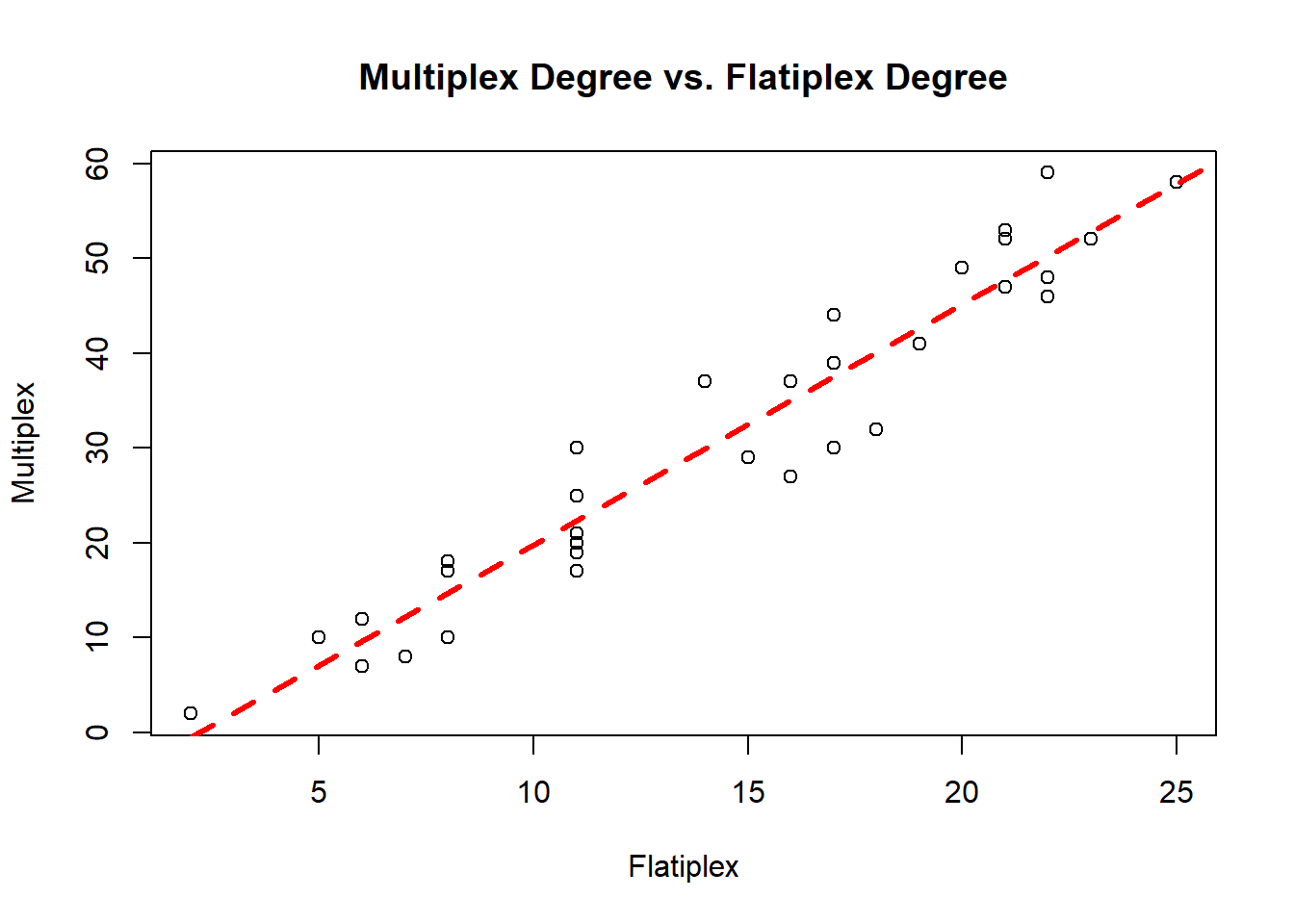
# What about the degree distribution?
par(mfrow = c(2,1))
hist(ml.deg, main = "Multiplex Degree Distribution")
hist(fl.deg, main = "Flatiplex Degree Distribution")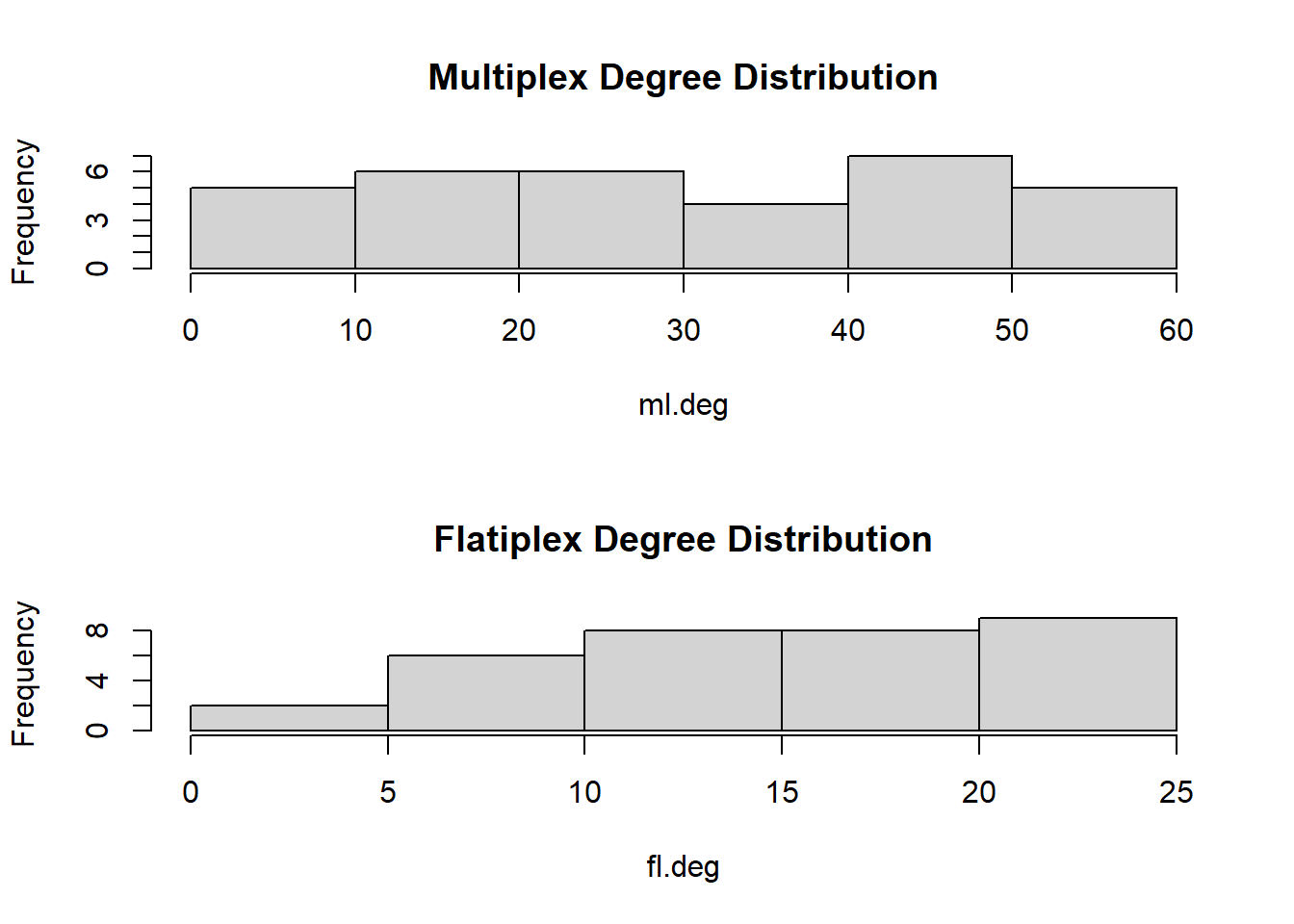
Since theflatjack is a weighted network, what if we measured strength instead of degree?
(fl.str = strength(theflatjack)) anxiety appetite_gain appetite_loss
52 7 44
difficulty_trusting emotional_numbness excessive_worry
39 47 19
fatigue fear_of_failure feeling_overwhelmed
48 18 17
feelings_of_detachment flashbacks guilt
48 32 21
hopelessness hypersomnia hypervigilance
10 17 12
insomnia intrusive_thoughts irritability
37 27 25
loss_of_interest low_energy low_self_esteem
52 30 10
nightmares psychomotor_retardation restlessness
49 37 30
rumination sadness somatic_complaints
46 58 41
suicidal_thoughts tearfulness weight_gain
59 8 53
weight_loss worthlessness panic_attacks
20 29 2 mod2 = lm(ml.deg ~ fl.str)
summary(mod2) Warning in summary.lm(mod2): essentially perfect fit: summary may be unreliable
Call:
lm(formula = ml.deg ~ fl.str)

Residuals:
       Min         1Q     Median         3Q        Max
-2.441e-15 -4.841e-16 -1.299e-16  1.498e-16  2.919e-15

Coefficients:
             Estimate Std. Error   t value Pr(>|t|)
(Intercept) 0.000e+00  3.919e-16 0.000e+00        1
fl.str      1.000e+00  1.100e-17 9.088e+16   <2e-16 ***
---
Signif. codes:  0 '***' 0.001 '**' 0.01 '*' 0.05 '.' 0.1 ' ' 1

Residual standard error: 1.034e-15 on 31 degrees of freedom
Multiple R-squared:      1, Adjusted R-squared:      1
F-statistic: 8.26e+33 on 1 and 31 DF, p-value: < 2.2e-16plot(fl.str, ml.deg,
xlab = "Flatjack",
ylab = "Multiplex",
main = "Multiplex Degree - Flatiplex Strength")
abline(mod2, lty = 2, lwd = 3, col = "red")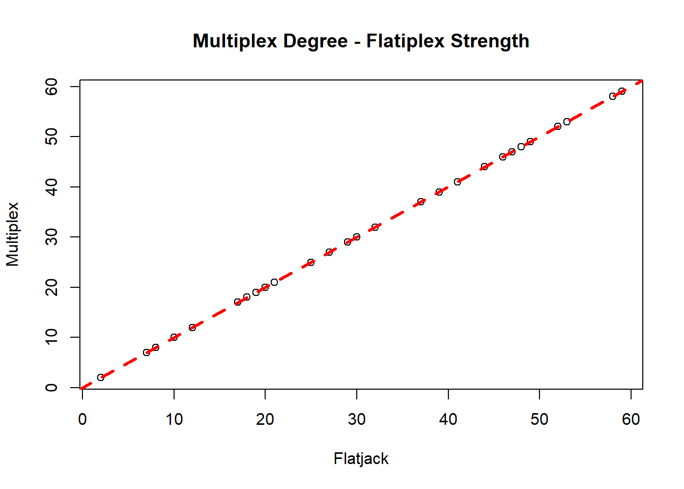
# What about the strength distribution?
par(mfrow = c(2,1))
hist(ml.deg, main = "Multiplex Degree Distribution")
hist(fl.str, main = "Flatiplex Strength Distribution")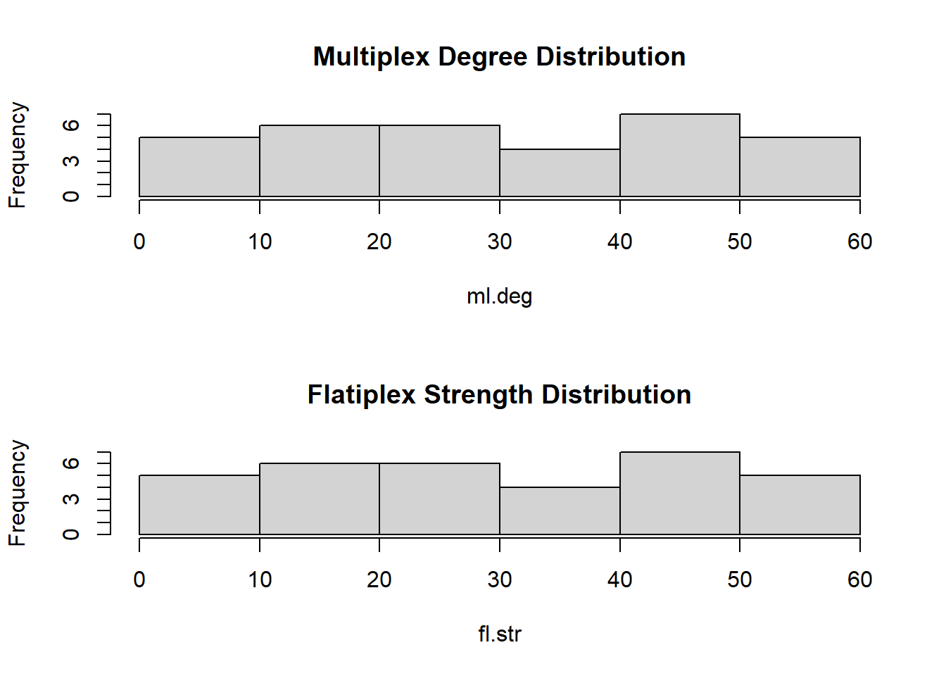
What about testing the distributions?
is.pl1 = displ$new(ml.deg)
is.pl1$setXmin(estimate_xmin(is.pl1))
bs1 = bootstrap_p(is.pl1, no_of_sims = 1000, threads = 20)
Expected total run time for 1000 sims, using 20 threads is 6.36 seconds.bs1$p[1] 0.704is.pl2 = displ$new(fl.deg)
is.pl2$setXmin(estimate_xmin(is.pl2))
bs2 = bootstrap_p(is.pl2, no_of_sims = 1000, threads = 20)Expected total run time for 1000 sims, using 20 threads is 2.99 seconds.bs2$p[1] 0.01Unlike standard degree, we can also get an idea of the variance between layers. Individuals with higher values vary more in between layers in their connections relative to others.
degree_deviation_ml(net) [1] 0.800000 2.800000 3.666061 6.019967 5.200000 7.391887 1.854724 2.785678
[9] 7.735632 6.305553 4.472136 2.638181 3.867816 1.959592 1.854724 4.874423
[17] 3.249615 5.176872 6.406247 2.993326 2.828427 4.758151 1.414214 2.280351
[25] 5.161395 2.607681 5.678028 2.576820 5.607138 2.059126 1.959592 4.833218
[33] 4.261455We can also inspect specific layers:
degree_ml(net, layers = "neural") [1] NA NA 6 6 7 15 NA 9 15 14 NA 9 12 NA NA 15 12 NA 5 4 NA 7 2 NA 12
[26] 9 14 8 9 4 4 10 4Or a subset of layers:
degree_ml(net, layers = c("neural", "genetic")) [1] NA 5 17 20 13 27 5 14 34 27 10 16 19 5 5 25 25 12 24 13 8 13 6 6 29
[26] 17 31 19 27 9 10 26 17We can check the neighborhood of each node:
neighborhood_ml(net) [1] 2 11 14 22 16 22 7 11 25 20 11 17 17 6 6 19 22 17 23 11 11 18 5 8 21
[26] 11 21 16 21 8 8 22 15as well as the redundancy of the graph given by:
1 - (Neighborhood / Degree)
connective_redundancy_ml(net) [1] 0.0000000 0.3529412 0.6216216 0.5416667 0.4074074 0.5416667 0.1250000
[8] 0.4761905 0.5689655 0.5918367 0.5600000 0.5641026 0.6136364 0.1428571
[15] 0.5000000 0.5365854 0.6271186 0.4333333 0.5576923 0.4210526 0.4500000
[22] 0.4375000 0.5000000 0.2000000 0.5961538 0.6333333 0.5531915 0.5675676
[29] 0.6037736 0.5555556 0.5294118 0.5217391 0.4827586Closeness
In a single-layer network, closeness is a centrality measure based on the shortest paths between nodes. It quantifies how “close” a node is to all other nodes, often defined as the inverse of the average shortest path length from that node to all others.
To extend this to multilayer networks, the concepts of paths and distances need to be generalized to account for connections that can span multiple layers. A path in a multilayer network can involve sequences of nodes and links, where links can be within or between layers. The length of a path can be defined in various ways. A simple definition is the number of edges. A more general definition assigns a weight to inter-layer edges, reflecting a ‘cost’ or difference in the nature of transitions between layers. The distance between two nodes is then the minimal length among all possible paths connecting them. Closeness can then be calculated based on these generalized shortest paths and distances in the multilayer structure.
The logic of this transformation is that a node’s ability to quickly reach other nodes might depend on its access to and position within different layers and the ease of transitioning between them. A node that is central in terms of reaching others through paths that utilize connections across multiple layers might be important in a different way than a node central only within a single layer. Different weighting schemes for inter-layer edges allow researchers to explore how varying the importance or cost of switching layers affects perceived closeness.
closeness(theflatjack) anxiety appetite_gain appetite_loss
0.01562500 0.01369863 0.01515152
difficulty_trusting emotional_numbness excessive_worry
0.01515152 0.01538462 0.01515152
fatigue fear_of_failure feeling_overwhelmed
0.01612903 0.01190476 0.01612903
feelings_of_detachment flashbacks guilt
0.01612903 0.01694915 0.01298701
hopelessness hypersomnia hypervigilance
0.01086957 0.01250000 0.01041667
insomnia intrusive_thoughts irritability
0.01190476 0.01694915 0.01190476
loss_of_interest low_energy low_self_esteem
0.01408451 0.01176471 0.01333333
nightmares psychomotor_retardation restlessness
0.01470588 0.01333333 0.01639344
rumination sadness somatic_complaints
0.01639344 0.01369863 0.01470588
suicidal_thoughts tearfulness weight_gain
0.01562500 0.01428571 0.01428571
weight_loss worthlessness panic_attacks
0.01492537 0.01470588 0.01234568 Clustering/Community Detection
In single-layer networks, community detection (or community inference/assignment) aims to partition nodes into groups (communities or modules) that are more densely connected internally than with nodes outside the group. Common methods are based on maximizing a quality function like modularity.
Community detection algorithms have been generalized to multilayer networks. These generalizations often involve extending the concept of modularity to account for the multilayer structure. Multilayer community detection algorithms offer flexibility, for instance, by allowing the possibility for different representations of the same node (node-tuples) to be assigned to the same or different communities across layers. The algorithms can be adjusted by parameters controlling the coupling between layers, influencing whether the assignment is biased towards grouping node-tuples of the same individual together (emphasizing consistent subgroups) or biased by connections within each layer (emphasizing differences across relationship types). This allows for identifying community structures that might span across multiple layers or reflect interdependencies between layers.
The logic of this transformation is to uncover mesoscale structures (communities) that are influenced by or exist across the various interaction types or contexts represented by different layers. It allows researchers to investigate whether communities are stable across different types of relationships or time periods, or if different interaction types define different community memberships for the same set of individuals. Adjusting layer coupling allows researchers to explore how different levels of interaction between layers influence the resulting community structure.
# Community Detection w/Louvain
  # General principle of Louvain is:
    # All vertices are their own community
    # Merge individuals based on who would improve Modularity the most
      # Repeat until no individual movements can be made to improve modularity
    # Generate a new adjacency matrix where group members form a larger, super-node
      # Each node has a new weight which is the sum of connections of all individuals in the
      # Community to the other communities
    # Repeat earlier steps until modularity no longer improves
set.seed(128673)
comm.struct.1 = glouvain_ml(net)
plot(net, com = comm.struct.1)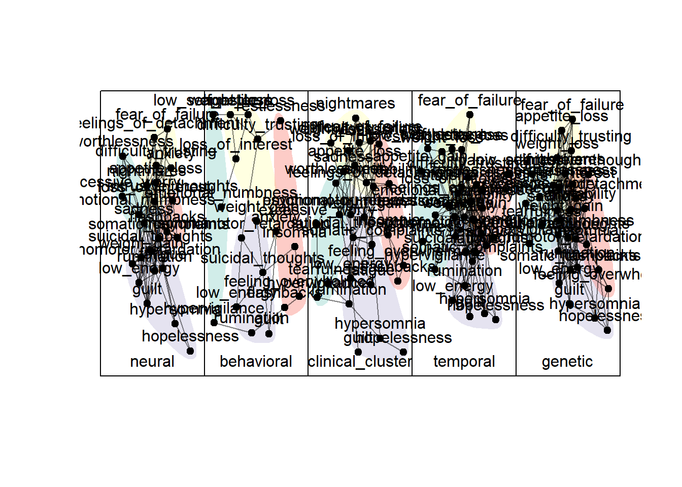
modularity_ml(net, comm.struct = comm.struct.1)[1] 0.4059366The results obtained from multilayer community detection are inherently different from single-layer methods. The ability for a multilayer algorithm to assign different node-tuples of the same individual to different communities is a capability not present in single-layer approaches, where each node belongs to only one community. This fundamental difference means that multilayer community detection reveals structures that cannot be captured by analyzing layers in isolation or by simple aggregation. Multilayer community inference methods facilitate quantifying components of social structure by assessing community structure over layers (interaction types, time windows), implying they capture patterns missed by single-layer analysis.
comm.struct.2 = igraph::cluster_louvain(theflatjack,
                                          weights = E(theflatjack)$weight)
# Examining ML Community Detection Results
comm.struct.1
actor layer cid
1 tearfulness clinical_cluster 0
2 tearfulness temporal 0
3 tearfulness genetic 0
4 sadness neural 0
5 sadness clinical_cluster 0
6 sadness temporal 0
7 sadness genetic 0
8 appetite_gain temporal 0
9 appetite_gain genetic 0
10 hypervigilance behavioral 0
11 hypervigilance clinical_cluster 0
12 hypervigilance temporal 0
13 hypervigilance genetic 0
14 excessive_worry neural 0
15 excessive_worry clinical_cluster 0
16 excessive_worry temporal 0
17 excessive_worry genetic 0
18 low_self_esteem behavioral 0
19 low_self_esteem temporal 0
20 low_self_esteem genetic 0
21 emotional_numbness neural 0
22 emotional_numbness behavioral 0
23 emotional_numbness clinical_cluster 0
24 emotional_numbness temporal 0
25 emotional_numbness genetic 0
26 worthlessness neural 0
27 worthlessness clinical_cluster 0
28 worthlessness temporal 0
29 worthlessness genetic 0
30 feelings_of_detachment neural 1
31 feelings_of_detachment clinical_cluster 1
32 feelings_of_detachment temporal 1
33 feelings_of_detachment genetic 1
34 nightmares neural 1
35 nightmares clinical_cluster 1
36 nightmares temporal 1
37 nightmares genetic 1
38 difficulty_trusting neural 1
39 difficulty_trusting behavioral 1
40 difficulty_trusting clinical_cluster 1
41 difficulty_trusting temporal 1
42 difficulty_trusting genetic 1
43 appetite_loss neural 1
44 appetite_loss behavioral 1
45 appetite_loss clinical_cluster 1
46 appetite_loss temporal 1
47 appetite_loss genetic 1
48 anxiety neural 1
49 anxiety behavioral 1
50 anxiety clinical_cluster 1
51 anxiety temporal 1
52 anxiety genetic 1
53 weight_loss behavioral 1
54 weight_loss clinical_cluster 1
55 weight_loss temporal 1
56 weight_loss genetic 1
57 loss_of_interest neural 1
58 loss_of_interest behavioral 1
59 loss_of_interest clinical_cluster 1
60 loss_of_interest temporal 1
61 loss_of_interest genetic 1
62 fear_of_failure neural 1
63 fear_of_failure clinical_cluster 1
64 fear_of_failure temporal 1
65 fear_of_failure genetic 1
66 fatigue neural 2
67 fatigue clinical_cluster 2
68 fatigue temporal 2
69 fatigue genetic 2
70 guilt neural 2
71 guilt behavioral 2
72 guilt clinical_cluster 2
73 guilt temporal 2
74 guilt genetic 2
75 somatic_complaints neural 2
76 somatic_complaints clinical_cluster 2
77 somatic_complaints temporal 2
78 somatic_complaints genetic 2
79 suicidal_thoughts neural 2
80 suicidal_thoughts behavioral 2
81 suicidal_thoughts clinical_cluster 2
82 suicidal_thoughts temporal 2
83 suicidal_thoughts genetic 2
84 hopelessness neural 2
85 hopelessness clinical_cluster 2
86 hopelessness temporal 2
87 hopelessness genetic 2
88 low_energy neural 2
89 low_energy behavioral 2
90 low_energy clinical_cluster 2
91 low_energy temporal 2
92 low_energy genetic 2
93 psychomotor_retardation neural 2
94 psychomotor_retardation behavioral 2
95 psychomotor_retardation clinical_cluster 2
96 psychomotor_retardation temporal 2
97 psychomotor_retardation genetic 2
98 weight_gain neural 2
99 weight_gain behavioral 2
100 weight_gain clinical_cluster 2
101 weight_gain temporal 2
102 weight_gain genetic 2
103 hypersomnia neural 2
104 hypersomnia clinical_cluster 2
105 hypersomnia temporal 2
106 hypersomnia genetic 2
107 rumination neural 2
108 rumination behavioral 2
109 rumination clinical_cluster 2
110 rumination temporal 2
111 rumination genetic 2
112 panic_attacks temporal 3
113 feeling_overwhelmed behavioral 3
114 feeling_overwhelmed clinical_cluster 3
115 feeling_overwhelmed temporal 3
116 feeling_overwhelmed genetic 3
117 insomnia neural 3
118 insomnia behavioral 3
119 insomnia clinical_cluster 3
120 insomnia temporal 3
121 insomnia genetic 3
122 intrusive_thoughts neural 3
123 intrusive_thoughts temporal 3
124 intrusive_thoughts genetic 3
125 irritability clinical_cluster 3
126 irritability temporal 3
127 irritability genetic 3
128 restlessness behavioral 3
129 restlessness clinical_cluster 3
130 restlessness temporal 3
131 restlessness genetic 3
132 flashbacks neural 3
133 flashbacks behavioral 3
134 flashbacks clinical_cluster 3
135 flashbacks temporal 3
136 flashbacks genetic 3comm.struct.1[comm.struct.1$cid == 1, ] actor layer cid
30 feelings_of_detachment neural 1
31 feelings_of_detachment clinical_cluster 1
32 feelings_of_detachment temporal 1
33 feelings_of_detachment genetic 1
34 nightmares neural 1
35 nightmares clinical_cluster 1
36 nightmares temporal 1
37 nightmares genetic 1
38 difficulty_trusting neural 1
39 difficulty_trusting behavioral 1
40 difficulty_trusting clinical_cluster 1
41 difficulty_trusting temporal 1
42 difficulty_trusting genetic 1
43 appetite_loss neural 1
44 appetite_loss behavioral 1
45 appetite_loss clinical_cluster 1
46 appetite_loss temporal 1
47 appetite_loss genetic 1
48 anxiety neural 1
49 anxiety behavioral 1
50 anxiety clinical_cluster 1
51 anxiety temporal 1
52 anxiety genetic 1
53 weight_loss behavioral 1
54 weight_loss clinical_cluster 1
55 weight_loss temporal 1
56 weight_loss genetic 1
57 loss_of_interest neural 1
58 loss_of_interest behavioral 1
59 loss_of_interest clinical_cluster 1
60 loss_of_interest temporal 1
61 loss_of_interest genetic 1
62 fear_of_failure neural 1
63 fear_of_failure clinical_cluster 1
64 fear_of_failure temporal 1
65 fear_of_failure genetic 1unique(comm.struct.1[comm.struct.1$cid == 1,]$actor)[1] "feelings_of_detachment" "nightmares" "difficulty_trusting"
[4] "appetite_loss" "anxiety" "weight_loss"
[7] "loss_of_interest" "fear_of_failure" # We see some overlap between Group 1 of ML and FL graphs:
comm.struct.2IGRAPH clustering multi level, groups: 4, mod: 0.19
+ groups:
$`1`
[1] "anxiety" "appetite_loss" "difficulty_trusting"
[4] "fear_of_failure" "feelings_of_detachment" "loss_of_interest"
[7] "nightmares" "weight_loss"
$`2`
[1] "appetite_gain" "emotional_numbness" "excessive_worry"
[4] "hypervigilance" "low_self_esteem" "sadness"
[7] "tearfulness" "worthlessness"
+ ... omitted several groups/verticesDiscussion Question
Define a few examples of systems we’ve discussed in the quarter that we treated as unipartite (one-dimensional) but could reasonably be recast as a multilayer or multiplex network