library(BoolNet)
library(igraph)PSC-190/290: Boolean Networks
Introduction (Psychological Data and Modeling)
Libraries
Regular graphs are binary {0,1}
- Consist of connections between nodes, yes connection (1) or no connection (0)
We can trivially extend this to continuous data
- We can utilize statistical methods such as k-means clustering to help split our data, which can subsequently be interpreted in binary form (k = 2).
- Weighted graphs can also be used to help represent the information or supplement our clustering.
- The nature of psychological constructs (ex. intelligence, psychological disorders, memory, etc.) means that continuous data is quite prevalent in psychology.
- We tend to prefer to describe these things on a spectrum rather than in categories.
Models of continuous data are much easier to imagine in psychology:
- Partial Correlation Networks: networks that account for weighted relationships between variables throughout a network.
- Dynamic Networks: networks that account for changes over time.
- Etc.
The study of psychology involves a lot of dynamic interactions between symptoms, personalities, biology, intelligence, etc. Continuous data enables more flexibility and better encapsulates how complex the human psyche is and how it is capable of changing over time.
Ising Model for cross-sectional data
In simple terms, the Ising model, designed for cross-sectional data is able to represent binary data in a network in terms of their probabilities at a single point in time.
- This is kind of like a “snapshot”
- Means that it is limited when it comes to:
- Making causal inferences
- Detecting dynamic changes or changes across time
- accurately modeling dynamic networks (like those commonly found in psychology)
Thus, here is the gap filled by Boolean networks which can model dynamical systems.
Boolean Networks
Context
Boolean networks have seen extensive usage in biology, largely to model gene regulatory networks as well as signal transduction pathways.
The onset of certain diseases can largely be traced back to irregularities in signal transduction pathways in the body, which in turn can be modeled by Boolean networks for analysis.
Boolean networks are particularly useful for understanding the structure of smaller-scale networks and for modeling dynamic relations within such networks.
(Albert and Robeva, 2015).
Introduction to Binary data
(Basic) Integers in Binary
Each respective place to the left represents the next power of 2.
Mathematically, this comes out to (\(2^n\)).
- 001 = 1
- 010 = 2
- 100 = 4
We can count up using similar rules to “normal” counting, once we get to the “maximum” number allotted we move places (ex. 9 \(\rightarrow\) 10) But instead we are counting by 0s and 1s instead of 10.
- Counting from 000 to 111
- 000 = 0
- 001 = 1
- 010 = 2
- 011 = 3
- 100 = 4
- 101 = 5
- 110 = 6
- 111 = 7
Question: What would “8” be in binary following these rules?
1000For our purposes this is just an introduction to binary integers for context, though more complex mathematical operations can be done.
Applications to Boolean Networks
Modeling a network in binary enables us to have a more digestible representation of often very complex interactions.
NOTE: A network with “\(n\)” nodes has a total possible \(2^n\) states
Boolean networks allow us to represent and organize all possible states in terms of “1s” and “0s” or whether a respective node is “ON” vs “OFF”.
Mathematically, a network with two nodes has 4 possible states.
Representing the nodes in terms of “1s” and “0s”, what are these 4 possible states?
00, 01, 10, 11Did you notice anything interesting about how we represented the states in relation to our discussion of binary integers?
Answer
We can represent them as decimals in order. “00” represents 0, “01” represents 1 and so forth. While the pattern of the digits is what we will see is significant in Boolean networks, decimal notation has potential merits for helping index and/or visualize data.Boolean Networks
Formulation
A Boolean Network can be represented by \[G = (X(t),B)\] Where X is a set of nodes at a time (t). \[ X = \{x_1(t), x_2(t), ..., x_n(t)\} \] And B is a set of functions. \[ B = \{f_1, f_2, ..., f_n\} \] These Boolean functions define the connections between the nodes using “AND”, “OR” and/or “NOT” operators.
(Yang et al., 2022)
Boolean rules
AND rules
The condition for the node’s state being on (1) at t + 1 is dependent on all input being on simultaneously.
\[x_1(t+1) = x_2(t) ∧ x_3(t)\]
- \(x_1\) is active at the next time step if \(x_2\) AND \(x_3\) are active
OR rules
The condition for the node’s state being on at t + 1 is dependent on any one of the input being on.
\[x_1(t+1) = x_2(t) ∨ x_3(t)\]
- \(x_1\) is active at the next time step if \(x_2\) OR \(x_3\) are active
NOT rules
The condition for the node’s state being on at t + 1 is dependent on the input being off, conversely, if the input is on, the node’s state will be off (0).
\[x_1(t+1) = ¬x_2\]
- \(x_1\) is active if \(x_2\) is inactive, or vice versa. More simply, \(x_1\) is the opposite of \(x_2\).
At its core Boolean logic boils down to these “simple” operations, though networks often use combinations of these functions to represent more dynamic systems.
NOTE: In this way, a Boolean network can be likened to a “ripple effect” where activation in one node propagates to one or multiple other nodes throughout the network and throughout subsequent time steps.
Try interpreting the following equation: \[x_1(t+1) = (x_1(t)∧x_2(t)) ∨ ¬x_3(t)\]
\(x_1\) at the next time step is on if \(x_1\) is on AND \(x_2\) is on OR if \(x_3\) is off.Truth table
table <- data.frame(
  x = c(0, 0, 0, 0, 1, 1, 1, 1),
  y = c(0, 0, 1, 1, 0, 0, 1, 1),
  z = c(0, 1, 0, 1, 0, 1, 0, 1),
  output = c(1, 0, 1, 0, 1, 0, 1, 1)
)
#manually creating a table to represent output given input

colnames(table) <- c("x_1", "x_2", "x_3", "output at t + 1")

table
x_1 x_2 x_3 output at t + 1
1 0 0 0 1
2 0 0 1 0
3 0 1 0 1
4 0 1 1 0
5 1 0 0 1
6 1 0 1 0
7 1 1 0 1
8 1 1 1 1Here I have manually created the truth table for the equation above. Our inputs \(x_1\), \(x_2\) and \(x_3\) correspond to our nodes at time t, and our output is at time t + 1. You can see the activation pattern for all 8 respective iterations of our 3 nodes.
Attractors
An attractor is indicative of the “long-term” behaviors of a network; a state / behavior in the network that repeats indefinitely
Over the course of time a dynamic system will tend to settle in this state as a result of the properties of Boolean Networks.
Types of Attractors
Fixed-point Attractors
- Are stable over time, a single state that “leads” to itself.
Limit Cycle Attractors
- Sequence of states
- Looping: [1,0,1] \(\rightarrow\) [0,1,0] \(\rightarrow\) [1,0,0] \(\rightarrow\) [1,0,1]
- Oscillating: [0,1,1] \(\rightarrow\) [1,1,0] \(\rightarrow\) [0,1,1]
More Complex Attractors
- More complex attractors that may be “chaotic” or defined by more complex loops also exist
What purpose do they serve?
- Attractors can reveal things about a dynamic system that can be useful in analysis or more, depending on the network.
- Long-term behavior
- Long-term behaviors that are “avoided”
- Stability (may stay at one point, oscillate between points, loop, etc.)
- Basins
Are they “useful”? How so?
- Long-term behaviors can help us better understand the system
- In psychology this may model how symptoms may tend to lead to certain outcomes and help guide interventions
- Long-term behaviors that are “avoided” may be behaviors / outcomes we WANT
- In psychology this may help us develop methods to guide treatment towards specific goals
- Stability
- Understanding the ways symptoms or behaviors stabilize over time may be key to diagnosing / treating psychological disorders
Basins
Basins refer to the nodes or states that are observed to “lead” to our attractors. These states will always include our attractor states but may also include other states.
They can be particularly useful for helping draw connections and analyzing how a set of initial conditions may lead to an outcome.
In psychology can you think of any basins of attraction and subsequent attractors?
An example of an attractor can be depression. A depressive state can be extremely difficult to exit. A set of conditions or basin states that may lead to this include environmental factors that cause chronic stress, such as social isolation. Behavioral habits such as sleeping and cognitive patterns that contribute to low self-esteem or negative thinking may all be basin states. Once someone “lands” in these basins we may tend to see them fall into a depressive state over time.Example
set.seed(2828)
# Generating a random "N-K"
# N = Number of Nodes
# K =
# 1. Degree of each new vertex
# 2. Average degree
# Depending on if topology is fixed/scale_free
# Or homogeneous
# Topology:
# Homogeneous = Erdos-Renyi Random Graph
# scale_free = Barabasi-Albert Power Law
N = 3
net = generateRandomNKNetwork(n = N, k = 2,
topology = "homogeneous",
linkage = "uniform",
functionGeneration = "uniform",
noIrrelevantGenes = FALSE,
simplify = TRUE)
net$genes = c("Eating", "Studying", "Crying")
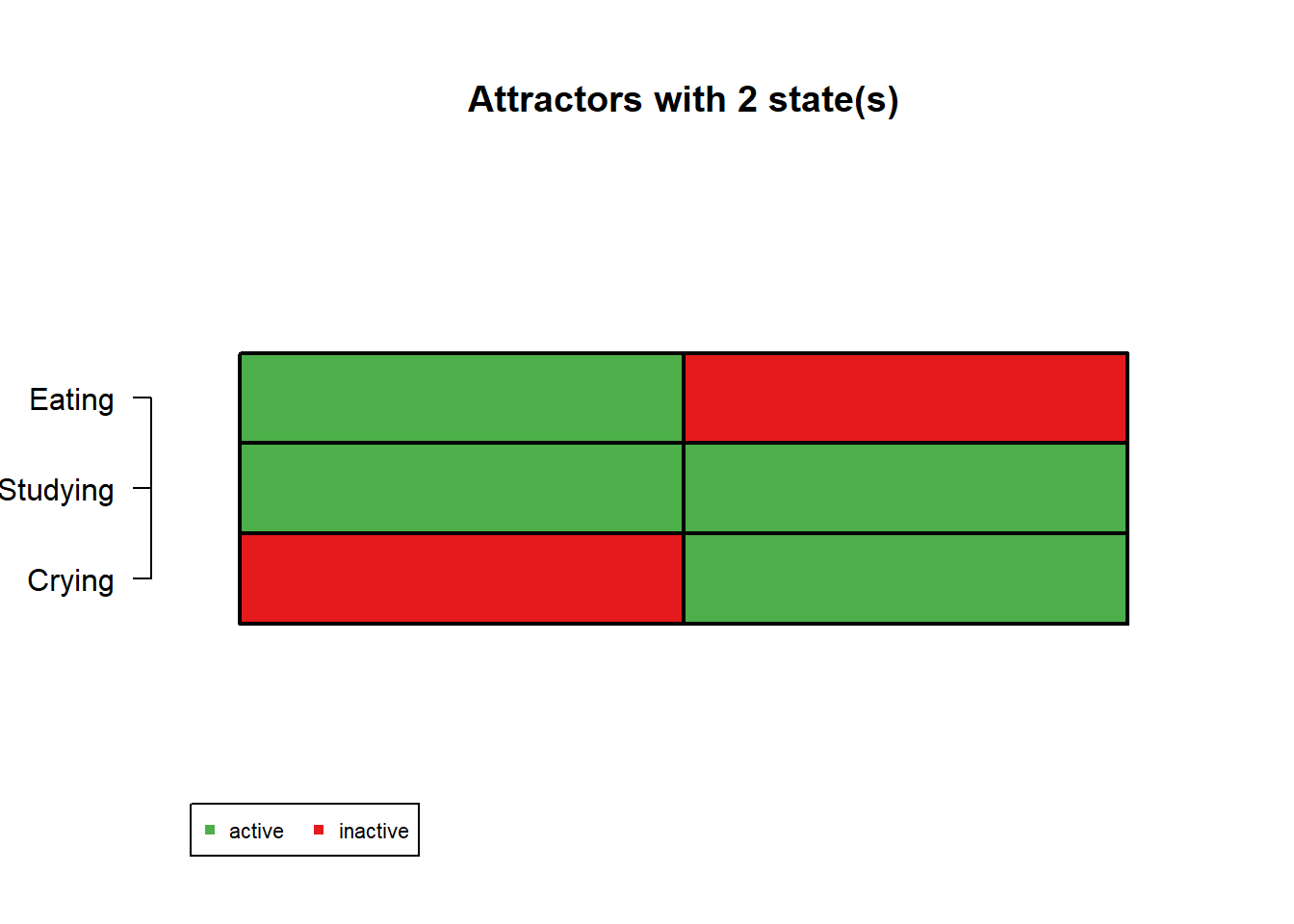
Attractors = getAttractors(net)
plotAttractors(Attractors)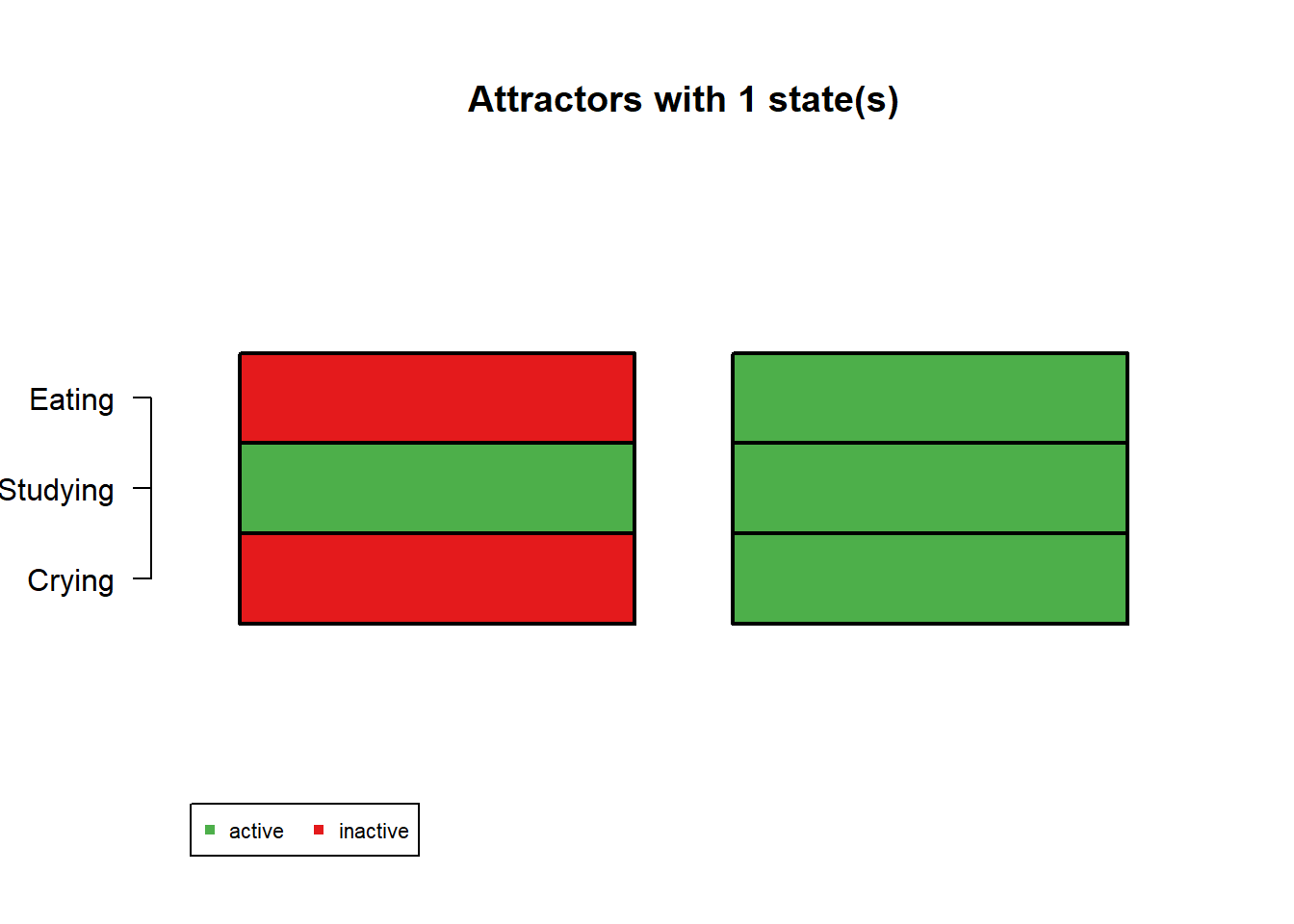
$`1`
         Attr1.1 Attr2.1
Eating         0       1
Studying       1       1
Crying         0       1

$`2`
         Attr3.1 Attr3.2
Eating         1       0
Studying       1       1
Crying         0       1
Interpretation
In this example we represent each of the nodes as an action.
- Node 1: Eating
- Node 2: Studying
- Node 3: Crying
Attractor 1 and 2 (single-state)
Attractors 1 and 2 are single-state attractors, meaning the network settles into a stable state upon entering either one of these states.
Attractor 1 may reflect a state in which you are a student and only studying, neglecting your nutrition but also not distressed and crying.
Attractor 2 may reflect a state in which you are a student who is studying, stressed and crying but also eating. Eating may also be related or due to stress though our model does not explicitly tie that in.
Attractor 3 (two-states)
- Attractor 3 may reflect a state in which studying is constant (maybe during a heavy exam week), that is, as a student you must be studying, though at times you may be eating and others, crying.
NOTE: It is possible for all 3 of these attractors to exist in the network, though the activation patterns of the network or the conditions for “landing” in these attractors may be different.
Now how can we apply this model to psychological data?
What about in Psychology?
Using the same random model:
 net$genes = c("Impulse control", "Emotional Response", "Behavioral Response")

 # Obtain the Steady-State Attractors of the Simulated Network
 Attractors = getAttractors(net)

 plotAttractors(Attractors)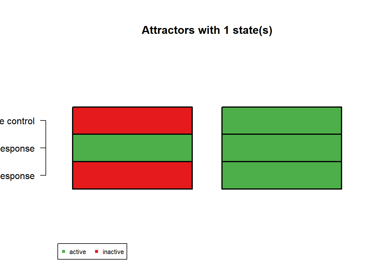

$`1`
                    Attr1.1 Attr2.1
Impulse control           0       1
Emotional Response        1       1
Behavioral Response       0       1

$`2`
                    Attr3.1 Attr3.2
Impulse control           1       0
Emotional Response        1       1
Behavioral Response       0       1
Interpretation
As an example, we can represent our random network as brain regions or mental processes responsible for certain actions.
- Node 1: Impulse Control
- Node 2: Emotionality
- Node 3: Behavioral Response
Attractor 1 and 2 (single-state)
Attractors 1 and 2 reflect stable states. They are separate single-state attractors, representing that our network is stable upon reaching either of these two states.
Attractor 1 may reflect a stable state in which impulse control is inhibited and behavioral response is inhibited, but emotionality is active. We can liken this to a state of high emotionality, where someone may be mentally overwhelmed and very emotional, and as a result unable to act on their emotions.
Attractor 2 may reflect a stable state in which impulse control is active, emotionality is active, and one’s behavioral response is also active. In this state, someone may be aware of their emotions and can act on them reasonably.
Attractor 3 (oscillating, two-states)
- Attractor 3 may reflect a state in which someone who struggles with controlling their impulses and behavioral response (oscillating between the two), and has high emotionality which may characterize psychological disorder.
Interestingly, in psychology, disorders are characterized largely by persisting patterns of behavior or thought. In our example, emotionality is the central component or node that is active.
AttractorsAttractor 1 is a simple attractor consisting of 1 state(s) and has a basin of 1 state(s):
|--<--|
V |
010 |
V |
|-->--|
Genes are encoded in the following order: Impulse control Emotional Response Behavioral Response
Attractor 2 is a simple attractor consisting of 1 state(s) and has a basin of 1 state(s):
|--<--|
V |
111 |
V |
|-->--|
Genes are encoded in the following order: Impulse control Emotional Response Behavioral Response
Attractor 3 is a simple attractor consisting of 2 state(s) and has a basin of 2 state(s):
|--<--|
V |
110 |
011 |
V |
|-->--|
Genes are encoded in the following order: Impulse control Emotional Response Behavioral ResponseNOTE: A network can have multiple attractors, and these attractors may differ by type, with a different number of basins
In our 3 node example, the basin size for Attractors 1 and 2 is 1. Meaning there is 1 possible state that makes our attractor state, corresponding to [0, 1, 0] and [1, 1, 1] respectively.
For Attractor 3, we have a basin size of 2 states. Meaning that two states are part of the attractor’s basin and form the attractor itself, oscillating back and forth. Those are [1, 1, 0] and [0, 1, 1].
NOTE: For this specific scenario, in our 3 node network, the basins themselves are the same as the attractors. It is entirely possible in larger more complex networks that the basins differ from the set of states of the attractors.
NOTE: More nodes in a network increases the potential basin size but does not directly mean that an attractor will have a larger basin size.
Application
How to do this in \(\texttt{R}\)
Generating Continuous Data
observed = generateTimeSeries(network = net,
                                numSeries = 1,
                                numMeasurements = 500,
                                type = "synchronous",
noiseLevel = 0.10) observed[[1]][, 1:20] 1 2 3 4 5
Impulse control 0.11822539 -0.12338907 0.03316483 0.03079127 0.08343707
Emotional Response 0.96332183 0.92144186 1.21272895 0.80973285 0.83397852
Behavioral Response -0.07859013 0.02927748 -0.06970263 -0.21746982 0.12751462
6 7 8 9 10
Impulse control 0.06643074 -0.01519009 0.1163749 -0.04610500 -0.09624696
Emotional Response 0.89051161 1.11059281 0.9676613 0.97645447 0.92715760
Behavioral Response 0.05268381 -0.05085016 -0.1243133 0.02303348 -0.08575196
11 12 13 14
Impulse control -0.003703682 0.05059863 -0.005634011 -0.011063985
Emotional Response 0.999517542 1.12848148 1.019844965 0.861546766
Behavioral Response -0.043764092 0.01849224 -0.008737934 -0.003898924
15 16 17 18 19
Impulse control -0.1042365 0.11718708 0.2209446 -0.08859233 -0.07841689
Emotional Response 0.9916840 1.11560851 1.1161717 1.04943941 0.95909243
Behavioral Response -0.1184053 0.01340382 0.1596859 -0.04174276 0.01780913
20
Impulse control 0.0287327
Emotional Response 0.8844970
Behavioral Response 0.0446918Binarization of Continuous Data
This is a LOT of data. Often our data isn’t represented by binary states, so how can we adjust it to fit our model while still retaining some accuracy?
# Binarize the time series and compare

bin = binarizeTimeSeries(observed, method = "kmeans")$binarizedMeasurements bin[[1]][, 1:20] 1 2 3 4 5 6 7 8 9 10 11 12 13 14 15 16 17 18 19 20
Impulse control 1 0 1 1 1 1 0 1 0 0 0 1 0 0 0 1 1 0 0 1
Emotional Response 0 0 1 0 0 0 1 0 0 0 0 1 1 0 0 1 1 1 0 0
Behavioral Response 0 1 0 0 1 1 0 0 1 0 0 1 0 0 0 1 1 0 1 1Simplified Explanation of Binarization
There is good evidence from simulation studies supporting the accuracy of Boolean networks in modeling continuous scale dynamics (Yang et al., 2022)
How does this process accurately represent our data?
- Using a threshold!
- K-means clustering (applied with k = 2)
- We can binarize the data by determining high and low values through clustering
- Thereby binarizing our values across two dimensions (0,1)
- Distance-based threshold (not as simple as “if x is greater than __“)
- K-means clustering (applied with k = 2)
Transition Functions and State Transition Graphs
  recon = reconstructNetwork(bin,
                             method = "bestfit",
                             maxK = N-1,
                             returnPBN = FALSE,
                             readableFunctions = FALSE)
 recon
Probabilistic Boolean network with 3 genes
Involved genes:
Impulse control Emotional Response Behavioral Response
Transition functions:
Alternative transition functions for gene Impulse control:
Impulse control = <f(Emotional Response,Behavioral Response){0001}> (error: 234)
Alternative transition functions for gene Emotional Response:
Emotional Response = <f(Emotional Response){10}> (error: 236)
Alternative transition functions for gene Behavioral Response:
Behavioral Response = <f(Emotional Response,Behavioral Response){1000}> (error: 220) recon = reconstructNetwork(bin,
method = "bestfit",
maxK = N-1,
returnPBN = FALSE,
readableFunctions = TRUE)
reconProbabilistic Boolean network with 3 genes
Involved genes:
Impulse control Emotional Response Behavioral Response
Transition functions:
Alternative transition functions for gene Impulse control:
Impulse control = (Emotional Response & Behavioral Response) (error: 234)
Alternative transition functions for gene Emotional Response:
Emotional Response = (!Emotional Response) (error: 236)
Alternative transition functions for gene Behavioral Response:
Behavioral Response = (!Emotional Response & !Behavioral Response) (error: 220)Interpretation
Our transition functions reflect the state of our node as they depend on other nodes. In this case:
- Impulse Control at the next time step is dependent on Emotional Response AND Behavioral Response being on.
- Emotional Response at the next time step is dependent on the opposite of Emotional Response
- Behavioral Response at the next time step is dependent on Emotional Response AND Behavioral Response being off simultaneously.
# Generate a single realization of the reconstructed network given:
  # functionIndices: Which functions to use for the computation of the next gene [node]
    # If Gene 1 is given by multiple nodes then we'll just pick the first "rule"
  # dontCareValues: For genes with "don't care" (*) entries in their truth table
  #   This argument provides values (0 or 1) to fill in those unspecified entries.
  #   Must be a list of vectors, with each vector matching the number of * values for its corresponding gene.
  # readableFunctions: Controls how the transition functions are printed when the network is displayed.
  #     FALSE: Shows raw truth table results.
  singlenet = chooseNetwork(recon, functionIndices = rep(1, N),
                            dontCareValues = rep(1, N),
                            readableFunctions = FALSE)
  singlenet
Boolean network with 3 genes
Involved genes:
Impulse control Emotional Response Behavioral Response
Transition functions:
Impulse control = (Emotional Response & Behavioral Response)
Emotional Response = (!Emotional Response)
Behavioral Response = (!Emotional Response & !Behavioral Response) # We can obtain attractors of the singlenet network
# We can use 2 update schemes:
# Synchronous and Asynchronous
# They have much to do with modeling of slower processes
# Synchronous Updates:
# Assume that the state of the system is updated at each moment:
# Generally, will lead to simple attractors and stable systems
ga = getAttractors(network = singlenet,
type = "synchronous",
returnTable = TRUE)
gaAttractor 1 is a simple attractor consisting of 2 state(s) and has a basin of 8 state(s):
|--<--|
V |
100 |
011 |
V |
|-->--|
Genes are encoded in the following order: Impulse control Emotional Response Behavioral ResponseInterpretation of Synchronous Update
Here we have defined a network in which noddes update synchronously, that is, nodes update together at each time step (t + 1). We see in our output that there is a basin of 8 states, meaning there are 8 possible initial conditions that will lead to this attractor. We also see that our simple attractor loops between 2 states.
    # Asynchronous update randomly selects a node and updates it
    # Contingent on the state of the system at the moment it is updated
  # Aysnchronous updates will identify the same states as a synchronous update
    # Can also find complex or "loose" attractors that govern a system
    ga2 = getAttractors(network = singlenet,
                      type = "asynchronous")
  ga2
Attractor 1 is a complex/loose attractor consisting of 8 state(s) and 18 transition(s):
111 => 110
111 => 101
011 => 010
011 => 001
011 => 111
101 => 100
101 => 111
101 => 001
001 => 000
001 => 011
110 => 100
110 => 010
010 => 000
100 => 101
100 => 110
100 => 000
000 => 001
000 => 010
Genes are encoded in the following order: Impulse control Emotional Response Behavioral ResponseInterpretation of Asynchronous Update
Asynchronous updates means that our nodes do not necessarily update together at the same time step, rather there is often more variation.
In this case we have a loose attractor which consists of 8 states but 18 resulting transitions.
This attractor type is not deterministic, meaning one state does not necessarily lead only to one other state, rather we can see some states have multiple possible outcomes. As a result it does not “loop” as attractors in previous examples have.
State Transition Graph
A State Transition Graph can enable us to visualize the multi-stability of Boolean Networks (Yang et al., 2022)
  # The above attractor is complex and consists of 8-states
    # Once the Boolean network enters any of these 8-states, it is trapped
    # The attractor will repeat indefinitely through time
    # But wait, we have 2^N possible states = 8 possible states
      # That means that this attractor is one in which the entire system cycles through indefinitely!
# Now, we can plot the state transition graphs
  # Credit to Xiao Yang for this plotting code
  p = plotStateGraph(ga, piecewise = TRUE,
                     drawLabels = T, plotIt = F,
                    colorsAlpha = c(colorBasinsNodeAlpha    = 1,
                                    colorBasinsEdgeAlpha    = 1,
                                    colorAttractorNodeAlpha = 1,
                                    colorAttractorEdgeAlpha = 1))
  plot.igraph(p, margin = 0.01,
              label.cex = 1,
              vertex.label.color = "black",
              vertex.label.dist = 2,
              remove.loops = TRUE,
              edge.arrow.size = 0.40)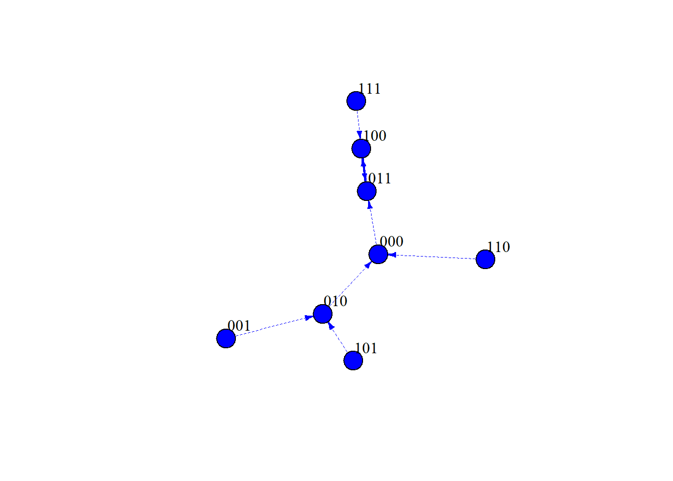
Interpretation
This State Transition Graph illustrates the dynamics of our 3 node network. Notice how in our graph, our edges are directed.
What is our attractor?
[1,0,0] \(\leftrightarrow\) [0,1,1], it seems to be an oscillating attractor in which any initial condition in this network will lead to this state eventually.
NOTE: It may take longer to get there from certain nodes.
Interpreting in the context of our example, it seems our stable state involves oscillation between high impulse control but no emotionality or behavior response, and high emotionality and behavior response but less impulse control.
In terms of overall behavior this may reflect our day-to-day interactions as people, we often go between rational and logical thinking and emotional reactions.
How many basin states are there?
- Every state in this network eventually leads into the oscillating attractor, including the states that define the attractor itself. Therefore, there are \(2^n\) basin states where n = 3.
Network Control and Boolean Networks for Psychological Research
Network Control
The broader purpose of network control in the context of Boolean Networks is to utilize the information we have on attractors to guide the network from undesireable attractors to more desireable outcomes (Yang et al., 2022).
- Using State Transition Graphs
- Using the knowledge obtained from state transiton graphs we can attempt to modify behavior depending on which nodes we deem to be the most influential.
- In the context of psychology, to try to guide people away from negative thinking patterns we may target sleeping habits or other health related habits if we deem those to have an influential effect on our target.
Yang et al. (2022) details a general procedure for identifying a control strategy:
- Formulating a goal of network control through identifying desireable and undesireable attractors
- Computing the Hamming distance between attractor and basin
- In simple terms, we want to know which nodes need to be manipulated
- As we know basins “lead” to attractors, we know the system will go to the attractor if it’s state is that of the attractor basin.
- The Hamming distance refers to the methodology via which this is done
- The distance between two states is just the amount of digits in which they differ
What is the Hamming Distance between [1,0,1,1] and [0,1,1,1]?
2, they only differ in the first two digits.- Identifying Control Strategies
- Determining which nodes affect the differences in Hamming distance enables us to figure out a way to manipulate that node in hopes of moving the system away from the undesireable state.
- Formulating Boolean functions to alter the behavior of the network
- We can subsequently define a function to direct the system from undesireable to desireable.
Usages in Psychology
As briefly mentioned before, data from Boolean networks can be used to create targeted treatment guiding the network towards desireable attractors.
- In psychology, we can target nodes that may represent specific symptoms to guide the network towards desireable outcomes.
It is also worth mentioning that we can also target the connections themselves. Campbell and Albert (2019) touches upon the idea of “Edgetic Perturbation” for use in biology. In cases where it may be difficult to completely eliminate certain nodes, altering the strength or disrupting the connections may be plausible for treatment.
- We can apply this idea to psychology as well, where it may not be feasible or appropriate to eliminate a symptom completely. Instead, we can figure out humane ways of enabling people to live with their symptoms and improve their overall quality of life.
Limitations and Concluding Remarks
Limitations
Some potential limitations to using Boolean networks include:
- Using Boolean networks to model on a large-scale may be incredibly computationally intensive and can be expensive
- Some data may not fit well in a binary model, data with a lot of noise may also be hard to adapt into a Boolean model
- It is hard to represent data that cannot be adapted well into binary data (ex. blood pressure)
- Some data may be very difficult to model with Boolean rules
Conclusion
Boolean networks have largely gained usage in the biological sciences for modeling gene regulatory networks and signal transduction pathways. Their usage is still limited within the field of psychology, though the application of Boolean networks may be useful for optimizing our analysis of networks of symptoms and other interactions for a wide variety of benefits.
- Its usage could create more personalized and smaller-scale models for diagnosis and treatment
- Boolean networks may also be incredibly useful for mapping and analyzing symptoms of psychological disorders to help with targeted treatment, similar to how they can reveal maladaptive nodes or irregularities in biological pathways.
Reflection/Discussion Questions
- What are your thoughts on the use of Boolean Networks to model psychological data, and when do you feel they are appropriate to use? Can you think of types of psychological data that would not be appropriately modeled by a Boolean network?
- Do you have any concerns about the use of Boolean Networks?
Transparency Statement
Some help from ChatGPT.