Adjacency Matrices

Adjacency Matrices

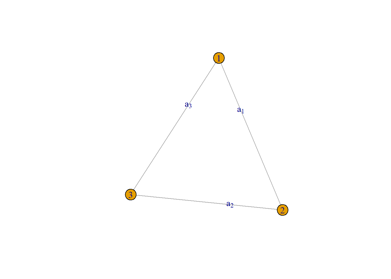
In graph theory, adjacency matrices are typically square matrices which are used to represent graphs. The elements of an adjacency matrix denote whether a set of vertices are linked or not. This means that the “cells” of an adjacency matrix are \(0.00\) when two vertices are not linked and \(1.00\) when they are linked.

There are cases when the links can be different from \(0.00\) or \(1.00\) and we’ll cover those next week.

The Adjacency of an Undirected Simple Graph

Let’s recall the original structure of our simple undirected graph:

\[G = (V,E)\]

where:

• \(G\): the graph is given by
• \(V\), a set of vertices and
• \(E \subseteq \{\{x, y\} \mid x, y \in V \text{ and } x \neq y\}\)

Recall, this basic graph:

• Forbids self-loops
• Is undirected

If we translate this to a matrix form, we get the following adjacency matrix:

\[ \underset{3\times 3}{\mathbf{A}} = \begin{bmatrix} 0 & a_{1} & a_{2} \\ a_{1} & 0 & a_{3} \\ a_{2} & a_{3} & 0 \end{bmatrix} \]

Notice that the diagonal elements are all 0. This aligns with the first argument that we cannot have self-loops. Also notice that certain cells have the same names. This is because each link between vertices can only happen once and is undirected.

Reflection.

• Given this adjacency matrix, what is the cardinality of the vertex set, \(V\)?
• What is the total possible cardinality of \(E\)?
• What type of matrix is \(\mathbf{A}\) other than square?

Answer.

• In this case, the cardinality of the vertex set (i.e., \(|V|\)) is the number of rows and/or columns of the adjacency matrix, \(\mathbf{A}\)
• 3; this is given by our past equation: \(|E|_{max} = \frac{|V|(|V|-1)}{2}\)
• \(\mathbf{A}\) is also symmetric. The values above and below the diagonal are equivalent

Let’s try creating the graph defined by this adjacency matrix:

library(igraph)
edges = c("1", "2",
          "2", "3",
          "1", "3")
g = make_graph(edges = edges, directed = FALSE)
E(g)$label = c(expression(a[1]), expression(a[2]), expression(a[3]))
plot(g)

See that the diagonal elements of an undirected graph is \(0.00\) because it forbids self-loops. Likewise, there are only 3-links aligning with our adjacency matrix.

Now, what about our digraph from earlier? What would the matrix of that look like? If we had the following defintion for our edges:

\[E \subseteq \{(x, y) \mid x, y \in V\}\]

• The links between vertices are no longer unordered pairs
• Self-loops are now allowed

This then generates the following adjacency matrix:

\[ \underset{3\times 3}{\mathbf{A}} = \begin{bmatrix} a_{1} & a_{2} & a_{3} \\ a_{4} & a_{5} & a_{6} \\ a_{7} & a_{8} & a_{9} \end{bmatrix} \] Notice that the diagonal elements are no longer \(0.00\) and the off-diagonal elements no longer match.

We can then create the resulting graph implied by this adjacency matrix:

edges = c("1", "1",
          "1", "2",
          "1", "3",
          "2", "1",
          "2", "2",
          "2", "3",
          "3", "1",
          "3", "2",
          "3", "3")
g = make_graph(edges = edges, directed = TRUE)
E(g)$label = c(expression(a[1]), expression(a[2]), expression(a[3]),
               expression(a[4]), expression(a[5]), expression(a[6]),
               expression(a[7]), expression(a[8]), expression(a[9]))
E(g)$curved = -0.3
plot(g, edge.arrow.size = 0.5)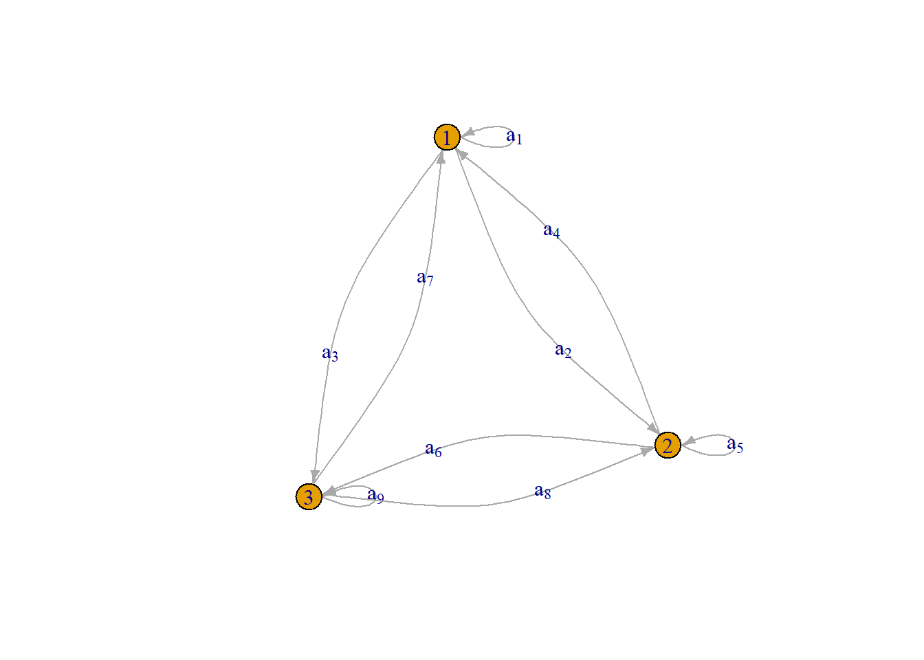

Notice that–unlike our simple undirected graph–this has 2 sets of links between each vertex pair and they have arrows denoting the direction of the association.

Reflection.

What networks have you seen or worked with that are digraphs? Perhaps more challenging, what networks do you think are more appropriate as undirected rather than directed graphs? Why?

“Powers” of the Adjacency Matrix

We end today’s meeting with a discussion on matrix exponents and the adjadency matrix. We already learned that for matrices to be multiplied against one another they must be “conformable”.

When we are exponentiating a matrix, conformability is not an issue because they are identical and therefore conformable.

An interesting property arises when exponentiating an adjacency matrix which is that \(\underset{n\times n}{\mathbf{A}}^k\) produces a matrix where each cell denotes the number of \(^{k}\) length paths or “walks” exist between two vertices. Let’s illustrate what that means with a simple example of a squared adjacency matrix:

\[ \underset{n\times n}{\mathbf{A}^{2}} = \begin{bmatrix} a_{11} & a_{12} & a_{13} \\ a_{21} & a_{22} & a_{23} \\ a_{31} & a_{32} & a_{33} \end{bmatrix} \] Here, the cell \(a_{21}\) would represent the number of 2-step paths that connect the two vertices in question. We can illustrate this more concretely with a larger graph:

set.seed(8391)
g = sample_pa(n  = 10, 
              power = 1.0,
              m = 2,
              directed = FALSE)
plot(g)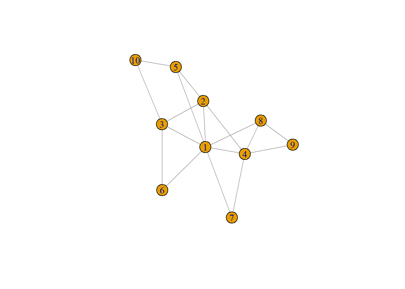

adj_matrix = as_adjacency_matrix(g, sparse = FALSE)
adj_matrix %*% adj_matrix

      [,1] [,2] [,3] [,4] [,5] [,6] [,7] [,8] [,9] [,10]
 [1,]    7    3    2    3    1    1    1    1    2     2
 [2,]    3    4    1    1    1    2    2    2    1     2
 [3,]    2    1    4    2    3    1    1    1    0     0
 [4,]    3    1    2    5    2    1    1    2    1     0
 [5,]    1    1    3    2    3    1    1    1    0     0
 [6,]    1    2    1    1    1    2    1    1    0     1
 [7,]    1    2    1    1    1    1    2    2    1     0
 [8,]    1    2    1    2    1    1    2    3    1     0
 [9,]    2    1    0    1    0    0    1    1    2     0
[10,]    2    2    0    0    0    1    0    0    0     2

To-Do’s for the Coming Week:

• Practice R and get familiar with \(\texttt{R}\)
• Read the assigned papers for this coming week
• Write your first weekly reflection paper [due before class next week]

Finally, a minor challenge:

• Define a digraph that allows for multiple connections between a set of vertices

Some graphs have properties that are unlike those we covered today. One such graph is the bipartite graph which–in its simplest form–is a graph composed of two sets of vertices.

For example, we may have \(V_{1}\) which is a set of researchers and \(V_{2}\) which is a set of publications where \(V_{1} \cap V_{2} = \emptyset\). For regular humans, this translates to: The intersection of \(V_{1}\) and \(V_{2}\) contains no elements; that is, they share no parts.

• Given that, what would the definition of \(E\) look like for a simple bipartite graph?
• What real-world networks do you think could be bipartite graphs?

Don’t cheat! Try it out before clicking!

\(E\subseteq \{\{x, y\} \mid x \in V_{1}, y\in V_{2}\}\)

We may forgo \(x\neq y\) because \(x\) and \(y\) are in separate sets therefore they cannot be equal given the definition: \(V_{1} \cap V_{2} = \emptyset\)