library(GeneNet)
library(qgraph)
library(GGMnonreg)
library(corpcor)PSC-190: Psychological Networks
What are Psychological Networks
The model that represent psychological variables and their relationships as a network, with nodes representing variables and edges representing statistical connections.
What characteristics do “psychological” networks have that networks in other fields do/do not have?
- Latent vs. Observable Constructs Psychological networks often involve theoretical constructs (e.g., depression, anxiety, motivation) that are not directly observable, unlike networks in biology (e.g., protein interactions) or transportation (e.g., flight routes), where nodes represent concrete entities.
As a result, psychological networks typically model symptoms or behaviors as proxies for these latent traits.
- Node Ambiguity and Construct Validity Nodes in psychological networks often represent ambiguous, overlapping, or interrelated constructs (e.g., fatigue vs. lack of energy), which makes node definition non-trivial.
In contrast, nodes in fields like computer science or engineering tend to have clear, discrete definitions (e.g., servers, routers).
- Edge Interpretation Edges in psychological networks (especially in Gaussian graphical models or partial correlation networks) often reflect statistical associations, not causal relationships.
In contrast, in biological or social networks, edges may reflect causal or physical connections (e.g., synaptic links, social ties).
Gaussian Graphical Model
A statistical model that represents the conditional dependencies between multiple random variables using a graph. In this model, nodes in the graph represent random variables, and edges between nodes represent conditional dependencies, meaning the variables are not independent when other variables are considered.
In the model, nodes represent variables like symptoms, traits, or behaviors, and edges represent partial correlations between these nodes. And partial correlation is a statistical measure that quantifies the relationship between two variables that also affect of all other variables in the dataset. In other words, it tells you how two variables are related above and beyond their shared associations with other variables.
Now let’s assume a random variable \(X_i\) for \(i \in 1...n\) are normal distributed \(X_i \sim {N}(\mu_i, \sigma_i^2)\) so the vector \(X\) of \(n\) vector random variables \(X_i\) has a multivariate normal distribution. Now we have the definition as following:
\[ X_i \sim {\mathcal{N}}(\mu, \Sigma) \]
Where \(\mu\) is the mean of the distribution, and typically it’s equal to 0 since we want to make a null hypothesis to assume there is no effect and difference. But the most important thing I want to talk about is \(\Sigma\), which represent the variance-covariance matrix.
We go deep in this, we want the precision matrix \(K\), which is inverse of \(\Sigma\) such that \(K= \Sigma^{-1}\). Since we said our \(\mu\) should be 0 which the distribution is stantardized, partial correlation coefficients of two variables, given all other variables will shows as following:
\[ \mathrm{Cor}(Y_i,Y_j \mid_{y-(i,j)}) = - \frac{k_{ij}}{\sqrt{k_{ii}}\sqrt{k{jj}}}\]
Where in which \(k_{ij}\) denotes an element of K, and \(y-(ij)\) denotes the set of variables without i and j. So by given this patial correlation between i and j, we can denote each \(Y_i\) is node and have the edge connect between two variable.
Now Run the R code:
set.seed(10086)
# Generating True Model
  true.pcor = ggm.simulate.pcor(num.nodes = 10, etaA = 0.40)
# Generating Data From Model
  m.sim = ggm.simulate.data(sample.size = 100, true.pcor)
# Covariance implied by Data
CovMat = cov(m.sim)
CovMat [,1] [,2] [,3] [,4] [,5] [,6]
[1,] 0.81699688 0.41864341 -0.01588008 0.40241985 -0.21793709 0.13909732
[2,] 0.41864341 0.97134922 0.00551491 0.14119892 -0.08884932 0.16700895
[3,] -0.01588008 0.00551491 1.07596182 0.04463695 -0.53032570 0.21766150
[4,] 0.40241985 0.14119892 0.04463695 0.84626216 -0.14029157 0.10458996
[5,] -0.21793709 -0.08884932 -0.53032570 -0.14029157 0.95569808 -0.27304911
[6,] 0.13909732 0.16700895 0.21766150 0.10458996 -0.27304911 0.95826049
[7,] -0.24878333 -0.45391026 0.13158388 -0.17999934 -0.16175977 -0.02408413
[8,] 0.37987352 0.28976982 -0.02323725 0.18107449 -0.03985842 -0.24324484
[9,] 0.03076401 0.20192004 0.10550776 0.09282696 -0.11511440 0.11501794
[10,] -0.02232774 0.14456669 -0.11580483 0.03209994 0.40340004 0.36938004
[,7] [,8] [,9] [,10]
[1,] -0.24878333 0.379873518 0.03076401 -0.022327738
[2,] -0.45391026 0.289769821 0.20192004 0.144566690
[3,] 0.13158388 -0.023237249 0.10550776 -0.115804828
[4,] -0.17999934 0.181074488 0.09282696 0.032099941
[5,] -0.16175977 -0.039858419 -0.11511440 0.403400036
[6,] -0.02408413 -0.243244837 0.11501794 0.369380038
[7,] 0.96258631 -0.397430931 -0.34545046 -0.394618523
[8,] -0.39743093 1.272749234 -0.17313095 0.001718706
[9,] -0.34545046 -0.173130955 0.96952834 0.082270315
[10,] -0.39461852 0.001718706 0.08227032 1.144340092# Modeling the true correlations
g1 = qgraph(true.pcor)
Now let’s generates the model with raw precision matrix data:
# raw precision matrix demonstration
pcor.mat = cor2pcor(CovMat)
G.test = qgraph(pcor.mat)
Explaination of graph
Obtaining a sparse network, Extended Bayesian Information Criterion (EBIC)
It is a model selection criterion used to choose the best model that fit the data and Penalizes complex models with too many parameters. Here EBIC uses LASSO penalty to shrink some connection toward 0. In other word, LASSO is a regularization method to approach the goal of minimize the information criteria.
Estimating the EBIC Graphical LASSO Network Model
# Estimating the EBIC Graphical LASSO Network Model
EBICgraph = qgraph(CovMat,
                   graph = "glasso",
                   sampleSize = nrow(m.sim),
                   tuning = 0.5,
                   # penalty for sparsity, another parameter
                   # tuning = 0.0, becomes BIC
                   details = TRUE)
Use Null-hypothesis Significance Testing (NHST)
Now let’s try the classical way to calculate the partial correlation:
# Estimating the NHST Gaussian Graphical Model and Generating a Plot
NHSTgraph = ggm_inference(m.sim, alpha = 0.05)
g3 = qgraph(NHSTgraph$wadj)qgraph(g3)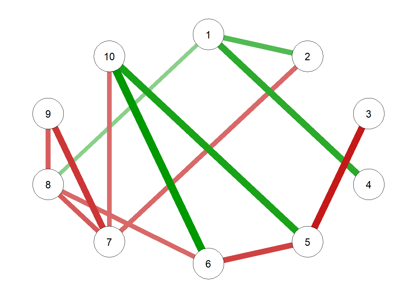
EBIC Regularization Evaluation
Now let’s see if our test is good regularization or not:
# Calculating the Layout Implied by the 3 graphs
  layout = averageLayout(g1, EBICgraph, g3)
# Calculating the maximum edge to scale all others to
comp.mat = true.pcor
diag(comp.mat) = 0
scale = max(comp.mat)Now we sets the edge widths based on the maximum connection, so all three graph use same scale, we can easy to compare them:
# Creating a Plot
  par(mfrow = c(3, 1))
  qgraph(true.pcor, layout = layout, theme = "colorblind",
         title = "True Graph", maximum = scale,
         edge.labels = round(true.pcor, 2))
  qgraph(EBICgraph, diag = FALSE,
         layout = layout, theme = "colorblind",
         title = "LASSO Graph", maximum = scale, edge.labels = TRUE)
  qgraph(NHSTgraph$wadj, layout = layout, theme = "colorblind",
         title = "NHST Graph", maximum = scale,
         edge.labels = round(NHSTgraph$wadj, 2))