# libraries
library(sna)
library(tsna)
library(ndtv)PSC-190: Temporal and Longitudinal Networks
Reviewing “Static” Networks
- So far, we’ve been covering static networks. In the context of temporal dynamics in psychology, a static network refers to a model that does not change over time. The relationships (edges) between elements (nodes) are assumed to be constant.
- Holme & Saramaki (2012) emphasize that in static networks, transitivity holds (if A → B and B → C, then A → C). In temporal networks, this property breaks down due to the importance of sequence and timing.
Static Networks in Psychological Temporal Dynamics
- Nodes often represent psychological variables (e.g., mood, anxiety, behavior).
- Edges represent associations (e.g., correlations, regressions) between these variables.
- In a static network, these associations are assumed to be stable across the entire study period.
Example: Pain, Sleep, and Mood
Imagine I ask you to model how pain, sleep, and mood relate to each other over a month.
In graph theory, a network is typically represented as a graph \[G =(V, E)\] where:
- V is the set of vertices (or nodes)
- E is the set of edges (or connections) between nodes
For this static psychological network:
- V = {Pain, Sleep, Mood}
- E consists of the statistical associations (e.g., partial correlations, regression coefficients) between these variables
Assume the data shows that:
Pain negatively affects Sleep (more pain → worse sleep)
Poor Sleep negatively affects Mood (less sleep → worse mood)
Pain also directly lowers Mood (more pain → worse mood)
An edge between Pain and Sleep (negative)
An edge between Sleep and Mood (positive)
An edge between Pain and Mood (negative)
These edges may be:
- Undirected (in correlation networks)
- Directed (in regression or causal models)
In a static network, these relationships are assumed to be stable across time.
What Are the Shortcomings of Static Networks?
Answer
While static networks offer a useful snapshot of psychological relationships, they come with important limitations:
No Temporal Resolution: They assume relationships are stable over time and miss fluctuations (e.g., stress might affect sleep differently across the week).
Events must follow time-respecting paths in temporal systems – something static representations can’t show (Pan & Saramaki, 2011).
No Directionality Without Assumptions: Undirected networks can’t tell us whether variable A affects B or the reverse.
Ignores Time-Lagged Effects: They miss how a variable today might influence another variable tomorrow (e.g., pain today → mood tomorrow).
Potential for Misleading Conclusions:
Question for Discussion
Suppose you’re studying the relationship between stress and mood. You collect data from each participant every day for one month.
What happens if you average stress and mood over time before analyzing their relationship?
Click to reveal answer
Averaging might hide short-term patterns. For example, if stress today lowers mood tomorrow, that time-lagged effect will be lost in the average, possibly leading to the (incorrect) conclusion that stress and mood are only weakly related.
Discuss the Element of Time
Introducing time into network models lets us move from static to temporal or longitudinal networks. These models:
- Allow time-lagged edges (e.g., Paint → Moodt+1), showing how earlier states affect later ones
- Distinguish within-person dynamics from between-person averages
- Reveal dynamic patterns like feedback loops, delays, and directional effects
- Require repeated measures (e.g., daily diaries or hormone sampling at multiple points throughout the day)
Static networks are like a snapshot. Temporal networks are like a movie.
Why Is Time Important?
It might seem like a silly question — but it’s critical to ask.
- Psychological processes are dynamic: They change from hour to hour, day to day.
- Timing clarifies causality: We can’t tell what leads to what without knowing when things happen.
- Symptoms have rhythms: Some issues (e.g., mood dips, anxiety spikes) follow a time-based pattern.
- We need time to see variation: Without repeated data, we miss how individuals fluctuate — and that’s where the real insight often is.
Introduce Temporal Networks
To build on the concept of a static network G = (V, E) — where V is the set of nodes and E is the set of edges — temporal networks add a new layer:
\[ G = (V, E, D) \] — where D stands for a temporal or dynamic dimension.
This extra layer allows us to represent how networks evolve through time. Each layer in D corresponds to a different time slice, and nodes or edges can appear, disappear, or change from one slice to another (e.g., mood today linked to sleep tomorrow) (Thompson et al., 2017).
Why G = (V, E, D)?
This allows us to capture not just who is connected, but also when. That timing is crucial for processes like:
Information flow
Disease transmission
Behavioral dynamics
Can you think of a real-world situation — in healthcare, education, or social life — where it’s critical to know when things happen, not just that they do?
For example, even if node A connects to B, and B to C, the order of those interactions determines whether a message can actually pass from A to C.
Compared to static closeness, temporal closeness is often more accurate for real-world systems — especially when timing and order matter.
Code Walkthrough: Temporal Network Construction & Analysis
Let’s say this dataset records interactions between people (e.g., students or patients)
- Each row = an interaction with onset/terminus (start/end times), and who was involved (tail/head)
- Could be social contact (epidemiology) or symptom co-occurrence (pain/sleep/stress)
#Read in data
 df <- read.csv("./df.csv")
  n_nodes = max(c(df$tail, df$head)) #Total number of unique nodes (people or symptoms)
#Create an empty undirected network
  base_net = network.initialize(n_nodes, directed = FALSE)
# Each row is a connection between two nodes (like two people or symptoms),
# with `onset` = when the connection started and `terminus` = when it ended.
# For example: edge between node 8 and 9 lasted from time 10 to 42.
# This means: at time 10, they interacted, and by time 42, that connection was gone.
# Edge duration is simply terminus - onset.
# R packages like `networkDynamic` require the data to be in this structure —
# a dataframe alone isn't enough; it must be converted into an object R understands as temporal.
# Example: Node 11 and 2 connected during three time intervals: 40–60, 80–120, and 130–181.
# In epidemiology, this tells us when and how people or symptoms came into contact,
# which helps trace influence, infection, or co-occurrence.
# Turn the edge list with onset/terminus into a temporal network
# Useful for modeling:
# - COVID spread among students (nodes = people)
# - Pain spreading between body parts or symptoms (nodes = symptoms)
net_dyn = networkDynamic(
base.net = base_net,
edge.spells = df[, c("onset", "terminus", "tail", "head")]
)Created net.obs.period to describe network
Network observation period info:
Number of observation spells: 1
Maximal time range observed: 10 until 300
Temporal mode: continuous
Time unit: unknown
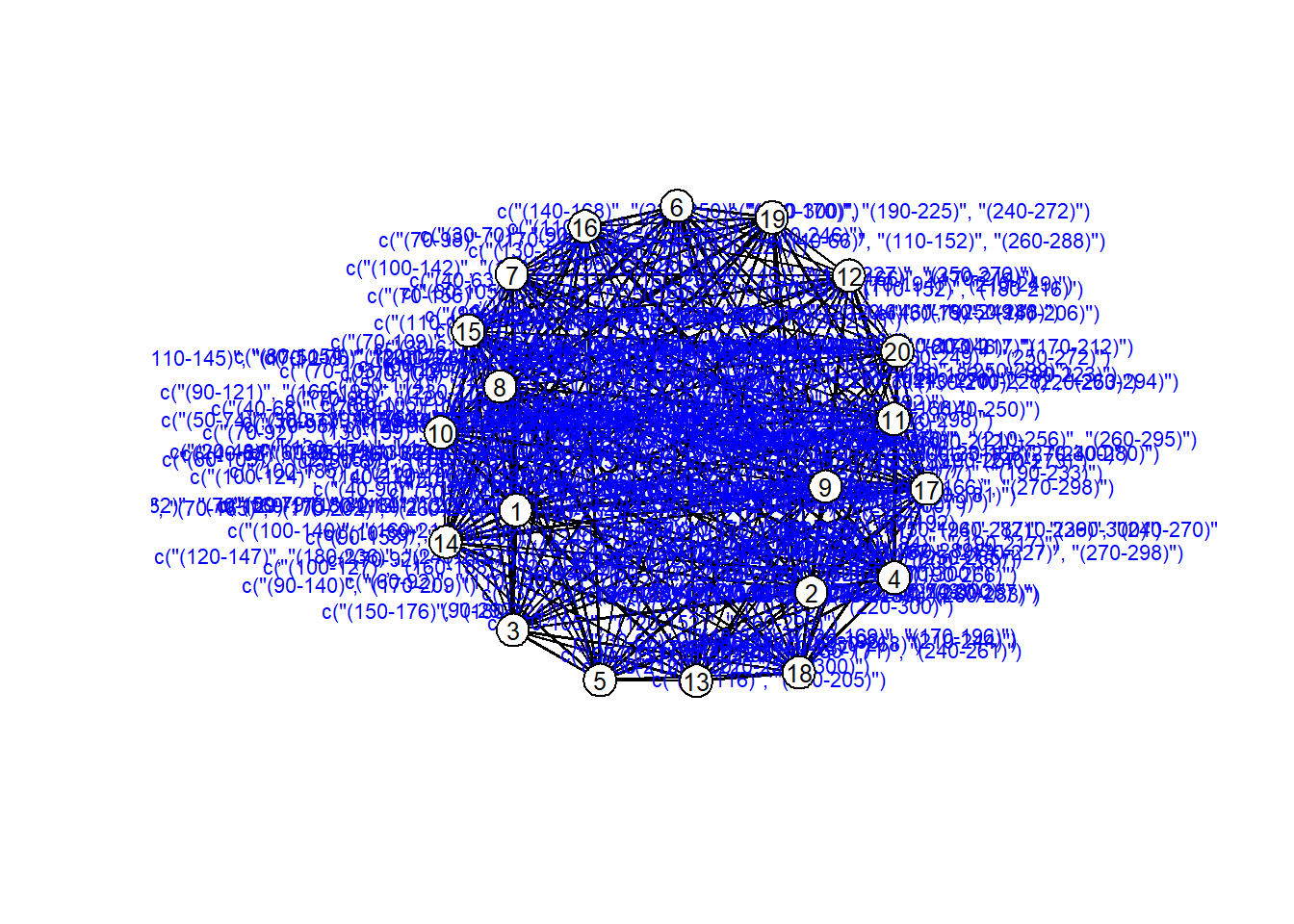
Suggested time increment: NA # Plot the network as a static layout (not time-aware)
# You can see who connects to whom, but you can't tell WHEN
# Helpful for checking layout and labels, but not great for time-based dynamics.
coords = plot(net_dyn,
displaylabels=TRUE,
label.cex = 0.8,
label.pos = 5,
vertex.col = 'white',
vertex.cex = 3,
edge.label = sapply(get.edge.activity(net_dyn),function(e){
paste('(',e[,1],'-',e[,2],')',sep='')
}),
edge.label.col = 'blue',
edge.label.cex = 0.7
)
Snapshot of the network at 4 different time points (like a film reel)
- helps visualize how interactions evolve over time ## Use cases:
- At t = 1: No one is sick yet (no edges).
- At t = 200: Major outbreak or symptom flare-up (dense network).
- At t = 300: Recovery or intervention - fewer interactions.
par(mfrow = c(2, 2))
  times = c(1, 100, 200, 300)
  titles = paste("Network at t =", times)
  invisible(lapply(seq_along(times), function(i) {
    plot(
      network.extract(net_dyn, at = times[i]),
      main = titles[i],
      displaylabels = TRUE,
      label.cex = 0.6,
      label.pos = 5,
      vertex.col = 'white',
      vertex.cex = 5,
      coord = coords
    )
     graphics.off()
  }))

# Or have R make it for you:
#Alternate way to think about this could be like a comic strip of a network changing.
filmstrip(net_dyn, frames = 4, displaylabels = FALSE)
Create a controllable animation showing how symptoms interact or disease spreads
# STEP 5: Compute animation frames for dynamic visualization
# Kamada-Kawai layout makes node movement smooth and visually consistent
compute.animation(
  net_dyn,
  animation.mode = "kamadakawai",
  slice.par = list(
    start = 1,
    end = 310,
    interval = 10,       # time steps between frames
    aggregate.dur = 10,  # collapse interactions within 10-step chunks
    rule = "any"         # include edges active at ANY point in each chunk
  )
)

  render.d3movie(
    net_dyn,
    output.mode = "htmlWidget",
    displaylabels = FALSE,
    # This slice function makes the labels work
    vertex.tooltip = function(slice) {
      paste(
        "<b>Name:</b>", (slice %v% "name"),
        "<br>",
        "<b>Region:</b>", (slice %v% "region")
      )
    }
  )
#Trace forward influence from one node (e.g., Patient Zero or Stress)
# tPath tells us:
# - How long it took to reach another node (tdist)
# --> # tdist: distance from t = origin for v to affect the i^{th} node
# - Who you were just with before arriving there (previous)
# --> # previous: The node that immediately preceeded landing on the i^{th} node
# - How many steps it took (gsteps)
# --> # gsteps: The number of "graph" steps to get to the i^{th} node
# In symptom networks: stress might trigger pain in 3 steps; in epidemics: how fast does disease spread?
v1path = tPath(net_dyn,v = 1, direction = "fwd")
print(v1path)$tdist
[1] 0 19 29 29 29 29 29 29 29 29 29 29 29 29 29 39 29 29 29 19
$previous
[1] 0 1 2 3 8 1 3 3 20 8 7 20 3 11 2 3 8 4 7 1
$gsteps
[1] 0 1 2 3 4 1 3 3 2 4 4 2 3 5 2 3 4 4 4 1
$start
[1] 1
$end
[1] Inf
$direction
[1] "fwd"
$type
[1] "earliest.arrive"
attr(,"class")
[1] "tPath" "list" plot(v1path,
coord = coords,
displaylabels=TRUE)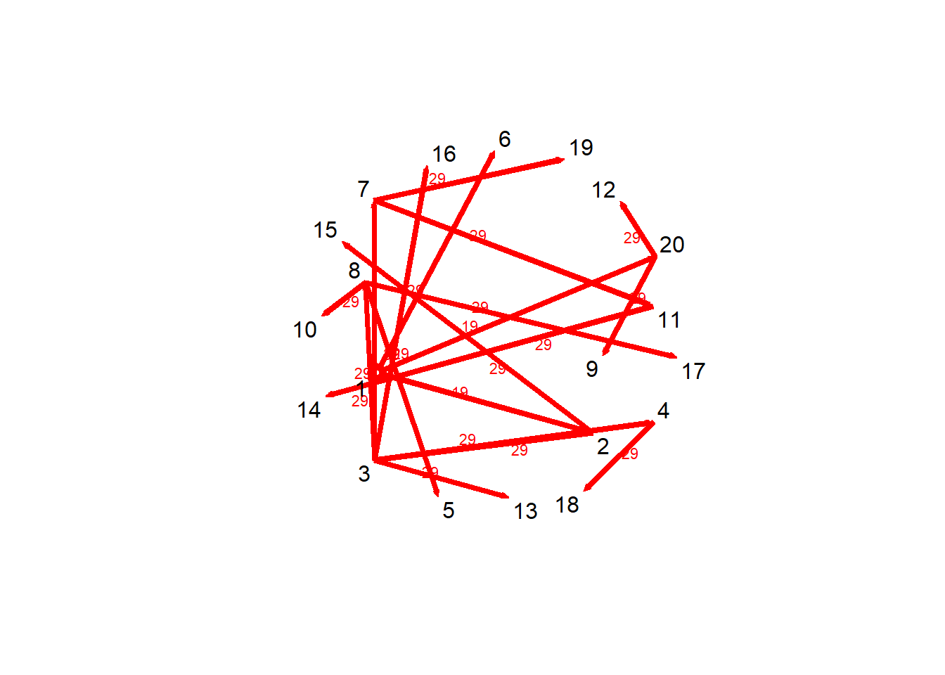
# Count how many edges are created at each time unit.
# Think: "How many new connections are forming every second/day?"
# Good for detecting when a wave of interactions/symptoms begins.
plot(tEdgeFormation(net_dyn, time.interval = 1))
Observing the number of connections as a function of time
#Graph Density over time — how interconnected the network is.
# A dense network means symptoms or people are all linked, signaling outbreak or flare-up.
# Helps quantify how connected a system is at a given time.
  plot(tEdgeFormation(net_dyn, time.interval = 1))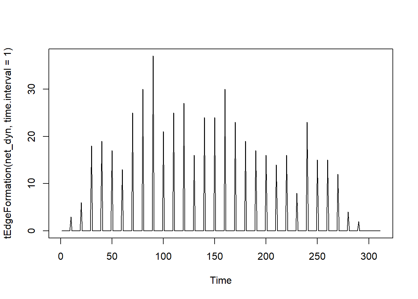
# Observing graph-based density as a function of time
  dynamicdensity = tSnaStats(
    net_dyn,
    snafun = "gden",
    start = 1,
    end = 300,
    time.interval = 1,
    aggregate.dur = 10
  )
  plot(dynamicdensity)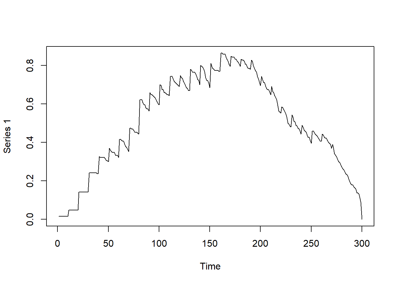
Observing betweenness in the graph over time
# Betweenness Centrality — identifies key 'bridge' nodes
# Who serves as the highway between disconnected clusters?
# In symptom networks: stress might bridge sleep and pain.
# In COVID: imagine one student who regularly visits both Floor A and Floor B in a dorm.
# While most people stay on their own floor, this student creates a link between two otherwise separate clusters.
# This makes them a potential 'bridge' for disease spread — a key node for transmission risk.
# In network terms, this node has high betweenness centrality because they sit on many shortest paths.
  dynamicbtw = tSnaStats(
    net_dyn,
    snafun = "centralization",
    start = 1,
    end = 300,
    time.interval = 1,
    aggregate.dur = 10,
    FUN = "betweenness"
    #maybe change FUN = degree
  )
  plot(dynamicbtw)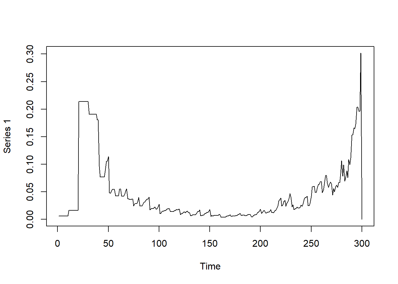
Dynamic Networks with AR(1) and VAR(1)
Now that we’ve explored how networks change visually and structurally over time, let’s turn to another approach: modeling the underlying processes that generate these changes.
These models help us understand how symptoms or variables influence each other over time, even when we can’t directly observe the causal system.
library(OpenMx)OpenMx functions for automatically fitting dt- and ct-var models Proprietary by Jonathan J. Park
-In the function below, you need N = 1 (single-subject) time-series data -You need variable names and may optionally specify the A, Q, and R matrices -They represent the dynamics, process noises, and measurement error variances, respectively -The equation for a state-space model is given by: ?mxExpectationStateSpace
\(State: x_{t} = A x_{t-1} + B u_{t} + q_{t}\)
\(Measurement: y_{t} = C x_{t} + D u_{t} + r_{t}\)
Which represent the state [dynamic] and space [measurement] equations
Applying these equations to a real world example:
- Imagine a patient is tracking their back pain level each day for a month as a part of a chronic pain study. The researchers want to model both:
- How the pain naturally evolves day to day (state process)
- How accurately the patient reports it (measurement process)
State Equation (latent):
- This equation describes how a person’s true pain level changes from one day to the next. It’s about what’s happening internally — even if we can’t see it directly.
- \(x_{t}\): patient’s true pain level today. –> This is a latent variable – it exists in reality, but we can’t observe it directly.
- \(x_{t-1}\): their true pain level yesterday –> Pain often carries over from day to day. That persistence is captured by A.
- \(u_{t}\): whether they took pain mediation (coded as 0 = no, 1 = yes)
- B: how medication affects pain
- \(q_{t}\): random influences on pain that we can’t control or measure –> Things like stress, poor sleep, weather – the unpredictable stuff.
You can think of the state equation as a behind-the-scences system: it tells us how pain unfolds over time, shaped by history and interventions.
Interpretation:
- Today’s pain depends on yesterday’s pain, the effect of medication, and random day-to-day variation.
Measurement Equation:
- This equation tells us how we actually observe the pain – for example, through a daily self-report score.
- \(y_{t}\): self-reported pain score (e.g., on 0-10 scale) –> This is what the person writes down or tells the researcher. -\(x_{t}\): the true pain at that time (from the state equation)
- \(C\): how closely true pain translates into reported pain –> Often set to 1, which could mean the person reports pain honestly and proportionally. –> Proportionally meaning that for every unit of true pain, the observed pain increases by a consistent amount. -\(r_{t}\) - random noise in what they report. –> Maybe they round up, minimize their pain, or misunderstand the scale.
The measurement equation connects the invisible (true pain) to the visible (what we measure). It reminds us that what we see may not be perfectly accurate.
  mx.var = function(dataframe = NULL, varnames = paste0('y', 1:nvar),
                    Amat = NULL, Qmat = NULL, Rmat = NULL){
    ne = length(varnames)
    ini.cond = rep(0, ne)
    if(is.null(Amat)){
      Amat = matrix(0, ne, ne)
    }
    if(is.null(Qmat)){
      Qmat = diag(1, ne)
    }
    if(is.null(Rmat)){
      Rmat = diag(1e-5, ne)
    }
    amat = mxMatrix('Full', ne, ne, TRUE, Amat, name = 'A')
    bmat = mxMatrix('Zero', ne, ne, name='B')
    cdim = list(varnames, paste0('F', 1:ne))
    cmat = mxMatrix('Diag', ne, ne, FALSE, 1, name = 'C', dimnames = cdim)
    dmat = mxMatrix('Zero', ne, ne, name='D')
    qmat = mxMatrix('Symm', ne, ne, FALSE, diag(ne), name='Q', lbound=0)
    rmat = mxMatrix('Symm', ne, ne, FALSE, diag(1e-5, ne), name='R')
    xmat = mxMatrix('Full', ne, 1, FALSE, ini.cond, name='x0', lbound=-10, ubound=10)
    pmat = mxMatrix('Diag', ne, ne, FALSE, 1, name='P0')
    umat = mxMatrix('Zero', ne, 1, name='u')
    osc = mxModel("OUMod", amat, bmat, cmat, dmat, qmat, rmat, xmat, pmat, umat,
                  mxExpectationStateSpace('A', 'B', 'C', 'D', 'Q',
                                          'R', 'x0', 'P0', 'u'),
                  mxFitFunctionML(), mxData(dataframe, 'raw'))
    oscr = mxTryHard(osc)
    return(ModRes = oscr)
  }
What’s the difference between AR and VAR
AR(1) - Auto-Regressive (one variable over time)
- One variable depends on its own past values
- Think of this like tracking just stress over time: –> How stressed was I today? –> How much of today’s stress can be predicted by yesterday’s stress?
EX - If someone has emotional inertia (like in depression), their mood today is heavily influenced by yesterday’s mood. That’s an AR(1) with a strong coefficient (e.g., 0.8)
Example 1: AR(1)
  ne = 1 #how many variables are there
  amat = mxMatrix('Full', ne, ne, TRUE, 0.80, name = 'A') #A matrix, full matrix, 1x1 matrix, give a true value of 0.8, name the matrix A)
  bmat = mxMatrix('Zero', ne, ne, name='B') #Matrix of means they are 0
  cdim = list("AR1", paste0('F', 1:ne)) #creating the C-matrix, diagnoal matrix (only values on the diagnoal nothing on the off diagnol .. diagnol is 1x1, FALSE - don't estimate, I know for a fact there is only one variable and that variable relates directly to my data)
  cmat = mxMatrix('Diag', ne, ne, FALSE, 1, name = 'C', dimnames = cdim) #fix the value at 1
  dmat = mxMatrix('Zero', ne, ne, name='D') # means for measurement model
  qmat = mxMatrix('Symm', ne, ne, FALSE, diag(ne), name='Q', lbound=0) #process noise co-variances, shocks in time, time error, symmetric, error variance is 1, called Q
  rmat = mxMatrix('Symm', ne, ne, FALSE, diag(1e-5, ne), name='R') #measurement error, going to be symmetric not estimating, diagnoal elements is 1 e-5 (because you cant set this to be 0, but need it to be very close, basically no measurement error)
  xmat = mxMatrix('Full', ne, 1, FALSE, 0, name='x0', lbound=-10, ubound=10)
  pmat = mxMatrix('Diag', ne, ne, FALSE, 1, name='P0')
  umat = mxMatrix('Zero', ne, 1, name='u')
  osc = mxModel("OUMod", amat, bmat, cmat, dmat, qmat, rmat, xmat, pmat, umat,
                mxExpectationStateSpace('A', 'B', 'C', 'D', 'Q',
                                        'R', 'x0', 'P0', 'u'))
  sim.data = mxGenerateData(osc, nrows = 1000)
  head(sim.data)
AR1
1 -0.4360536
2 -0.5641045
3 0.0706547
4 -0.1033369
5 -0.6473401
6 -1.6997582 plot(x = (1:nrow(sim.data)), y = sim.data$AR1, type = "l",
main = "Time-Series of AR1", ylab = "Values", xlab = "Time")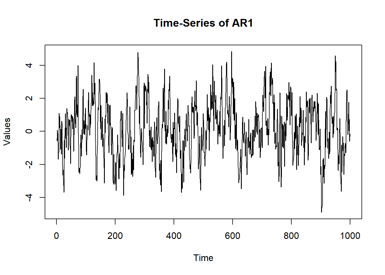
ar1 = mx.var(dataframe = sim.data, varnames = "AR1")Running OUMod with 1 parameter
Beginning initial fit attemptRunning OUMod with 1 parameter
Lowest minimum so far: 2853.61880723203
Solution found
Solution found! Final fit=2853.6188 (started at 4628.9621) (1 attempt(s): 1 valid, 0 errors) Start values from best fit:0.797491294722145 summary(ar1)$parameters name matrix row col Estimate Std.Error lbound ubound lboundMet
1 OUMod.A[1,1] A 1 1 0.7974913 0.01892778 NA NA FALSE
uboundMet
1 FALSE # Can compare to different AR:
osc$A$values = -0.80
sim.data = mxGenerateData(osc, nrows = 1000)
  plot(x = (1:nrow(sim.data)), y = sim.data$AR1, type = "l",
       main = "Time-Series of AR1", ylab = "Values", xlab = "Time")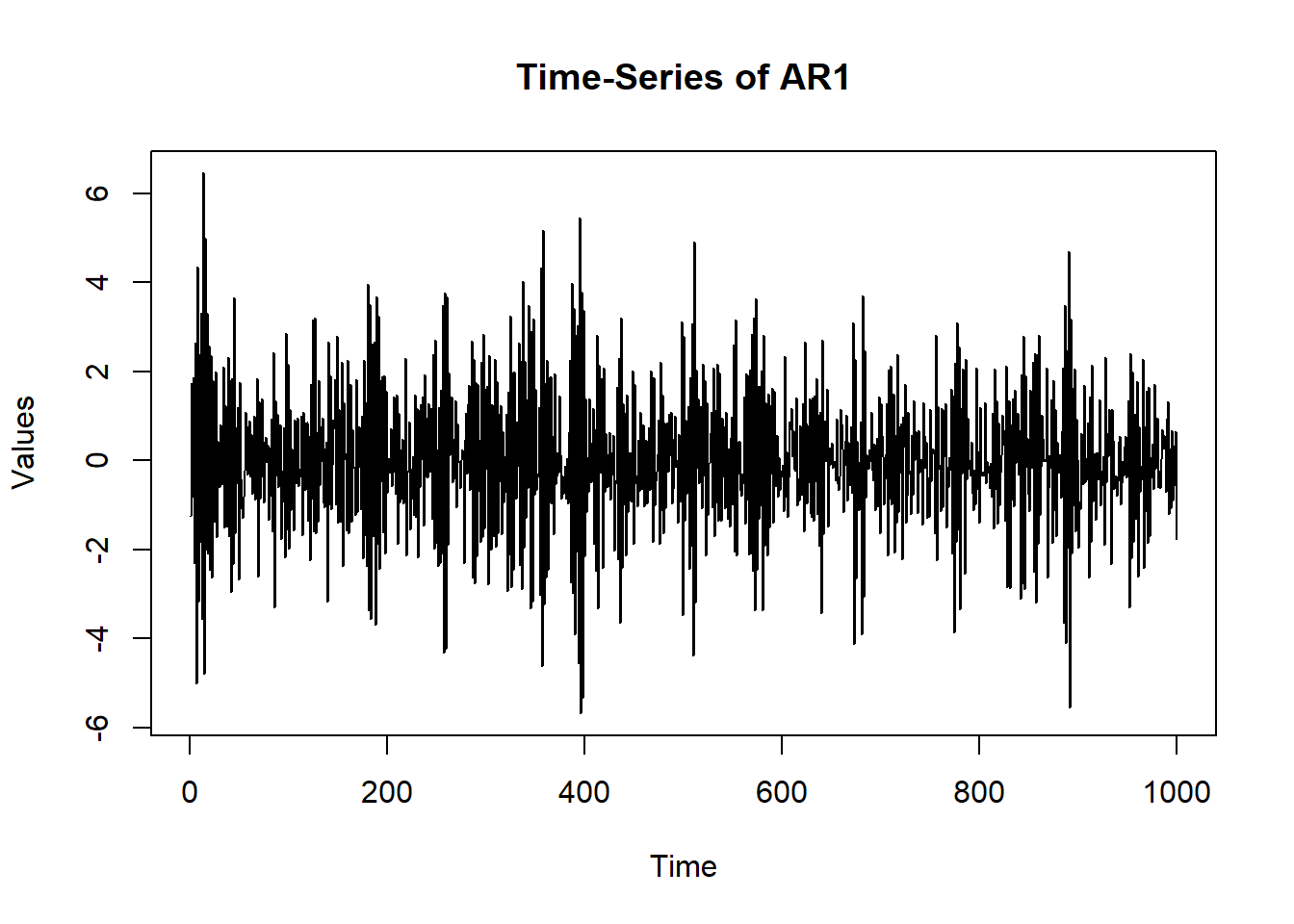
ar1 = mx.var(dataframe = sim.data, varnames = "AR1")Running OUMod with 1 parameter
Beginning initial fit attemptRunning OUMod with 1 parameter
Lowest minimum so far: 2836.72438604595
Solution found
Solution found! Final fit=2836.7244 (started at 4700.6888) (1 attempt(s): 1 valid, 0 errors) Start values from best fit:-0.807318795499414 summary(ar1)$parameters name matrix row col Estimate Std.Error lbound ubound lboundMet
1 OUMod.A[1,1] A 1 1 -0.8073188 0.01869848 NA NA FALSE
uboundMet
1 FALSEVAR(1) - Vector Auto-Regressive (multiple variables interacting over time)
- Each variable depends on past values of itself AND other variables
- Focuses on lagged relations – how past values predict future values ()
- Now imagine tracking stress, sleep, and pain over time
- Today’s stress depends on yesterday’s stress and sleep.
- Today’s sleep depends on yesterday’s sleep and pain.
- Today’s pain depends on yesterday’s pain and stress.
EX
- If stress affects pain, and poor sleep feeds back into stress – this creates a system. VAR(1) models capture this interconnected, dynamic relationship between multiple variables.
Comparing VAR, sVAR, and gVAR
(Gates & Liu, 2016; Park et al., 2020)
VAR (Vector Autoregression)
What it does: Looks at how each variable is affected by all the variables from the previous time point.
What it tells you: Shows how things from yesterday (like stress) can predict things today (like pain).
What it misses: Doesn’t show if two things (like stress and pain) happen together at the same time.
sVAR (Structural VAR)
What it does: Adds in the idea that some things can affect each other instantly, not just over time.
How it works: You have to decide which things can cause others right away (for example, you might say stress can immediately affect pain).
What you get: You see both the “yesterday-to-today” effects and the “right now” effects-but you need to make some assumptions about what causes what.
gVAR (Graphical VAR)
What it does: Similar to sVAR, but uses network diagrams to show relationships.
How it works: Draws lines between things that are connected at the same time (like mood and sleep), but doesn’t say which one causes the other.
What you get: Easy-to-read network maps that show which things are linked, both at the same time and over time.
  ne = 3
  VAR.params = matrix(c(0.60, 0.00, 0.00,
                        0.00, 0.60, -0.25,
                        0.25, 0.00, 0.60), ne, ne)
  amat = mxMatrix('Full', ne, ne, TRUE, VAR.params, name = 'A')
  bmat = mxMatrix('Zero', ne, ne, name='B')
  cdim = list(paste0("V", 1:ne), paste0('F', 1:ne))
  cmat = mxMatrix('Diag', ne, ne, FALSE, 1, name = 'C', dimnames = cdim)
  dmat = mxMatrix('Zero', ne, ne, name='D')
  qmat = mxMatrix('Symm', ne, ne, FALSE, diag(ne), name='Q', lbound=0)
  rmat = mxMatrix('Symm', ne, ne, FALSE, diag(1e-5, ne), name='R')
  xmat = mxMatrix('Full', ne, 1, FALSE, 0, name='x0', lbound=-10, ubound=10)
  pmat = mxMatrix('Diag', ne, ne, FALSE, 1, name='P0')
  umat = mxMatrix('Zero', ne, 1, name='u')
  osc = mxModel("OUMod", amat, bmat, cmat, dmat, qmat, rmat, xmat, pmat, umat,
                mxExpectationStateSpace('A', 'B', 'C', 'D', 'Q',
                                        'R', 'x0', 'P0', 'u'))
  sim.data = mxGenerateData(osc, nrows = 1000)
  head(sim.data)
V1 V2 V3
1 0.1426894 0.40123471 -0.9758537
2 -1.6073115 0.06366867 -0.8178305
3 -1.3573996 0.43444625 -0.2408048
4 -1.3267910 0.24261593 1.8042470
5 0.4345503 0.30669230 2.4607570
6 1.9066389 1.02512556 1.4666714 VAR1 = mx.var(dataframe = sim.data, varnames = paste0("V", 1:ne))Running OUMod with 9 parameters
Beginning initial fit attemptRunning OUMod with 9 parameters
Lowest minimum so far: 8508.38316348157
Solution found
Solution found! Final fit=8508.3832 (started at 11129.794) (1 attempt(s): 1 valid, 0 errors) Start values from best fit:0.60135268095721,-0.0496033631149735,-0.0180685822247098,-0.0039932113148108,0.642817898292957,-0.20855694829575,0.245842602222357,0.0170028588178409,0.627765566802595 summary(VAR1)$parameters name matrix row col Estimate Std.Error lbound ubound lboundMet
1 OUMod.A[1,1] A 1 1 0.601352681 0.02304798 NA NA FALSE
2 OUMod.A[2,1] A 2 1 -0.049603363 0.02304768 NA NA FALSE
3 OUMod.A[3,1] A 3 1 -0.018068582 0.02304981 NA NA FALSE
4 OUMod.A[1,2] A 1 2 -0.003993211 0.02520095 NA NA FALSE
5 OUMod.A[2,2] A 2 2 0.642817898 0.02520246 NA NA FALSE
6 OUMod.A[3,2] A 3 2 -0.208556948 0.02520427 NA NA FALSE
7 OUMod.A[1,3] A 1 3 0.245842602 0.02436166 NA NA FALSE
8 OUMod.A[2,3] A 2 3 0.017002859 0.02436266 NA NA FALSE
9 OUMod.A[3,3] A 3 3 0.627765567 0.02436387 NA NA FALSE
uboundMet
1 FALSE
2 FALSE
3 FALSE
4 FALSE
5 FALSE
6 FALSE
7 FALSE
8 FALSE
9 FALSE params = matrix(0, ne, ne)
for(i in 1:nrow(summary(VAR1)$parameters)){
params[summary(VAR1)$parameters[i,"row"], summary(VAR1)$parameters[i, "col"]] =
ifelse(abs(summary(VAR1)$parameters[i,"Estimate"]) > qnorm(0.975) * summary(VAR1)$parameters[i,"Std.Error"],
summary(VAR1)$parameters[i,"Estimate"],
0.00)
}
params [,1] [,2] [,3]
[1,] 0.60135268 0.0000000 0.2458426
[2,] -0.04960336 0.6428179 0.0000000
[3,] 0.00000000 -0.2085569 0.6277656 VAR.params [,1] [,2] [,3]
[1,] 0.6 0.00 0.25
[2,] 0.0 0.60 0.00
[3,] 0.0 -0.25 0.60Q&A
- How might the conclusions you draw from a static network differ if instead you used a temporal network? Can you think of a situation where knowing when a connection occurs is more important than just knowing thatit exists?
- If you had to monitor just one symptom or variable in a dynamic system (like mood, sleep, pain, or stress), which would you choose – and why?
- Do you think we should always model all variables, or can focusing on one or two lead to just as much insight?
- How could wearable data improve our ability to detect early warning signs for psychological distress or illness flare-ups? What challenges might we face in using this data reliably?