# libraries

library(sna)
library(tsna)
library(ndtv)PSC-290: Temporal Networks
Review of “Static” Networks
- Nodes (V) connected by edges (E) in one dimension of space or time. All the graphs we have discussed in the class so far are defined as: \[G = (V, E)\]
- Eg: Graphical Gaussian Models (GGMs), Ising Model that we discussed last week.
- These models have a ton of benefits. They are simple, and you can do a lot of interesting things with them. For example: calculate centrality indices to find “important” nodes; find clusters or communities in the nodes; use them to address specific hypotheses in psychology.
- You may use a static network to model the partial correlation network of symptoms of a patient. Using permutation techniques for NHST you can test if this network is significantly different from a neurotypical symptom network. If it is significantly different, maybe find a node/symptom that is a hub or if connected to a lot of other symptoms. Maybe intervening on this symptom is helpful?
- Having said that, static networks are limited!
What are their shortcomings?
Answer
- Aggregation loses temporal information (Thompson et al., 2017)
- GGMs, Ising Models represent individual moments/slices of time (from last week)
- Less suited for study of dynamical systems like information flow or brain activity (Holme & Saramaki 2012, Pan & Saramaki 2011, Thompson et al. 2017).
According to Emorie Beck, “I think all psychological phenomena are fundamentally about change. Even ‘fixed’ things like genetics are actually changing over time, so stability is an illusion!”
The Element of Time
How do you measure time? Is time truly continuous or discrete? Are psychological processes continuous or discrete? Are they necessarily smooth?
Introduction to Temporal Networks
How can time be represented in a static network?
So, we’ve established that time can be be a useful factor to take into account in a network. Temporal networks aim to capture this by adding another dimension, \(D\), to the base formula of a simple undirected graph. For today, the new dimension represented by \(D\) is time:
\[G = (V, E, D)\]
Graph \(G\) is given by set of vertices \(V\) and edges \(E\) at time \(D\). Here, \(D\) is a dimension of the network representing a given layer of the temporal network as a whole. Each layer is a different “slice” of time.
What types of data and/or research questions might be suited to this method of looking at “slices” of time? What may not be suited?
There are two main categories of temporal network (Holme & Saramaki 2012), contact sequences and interval graphs. Contact sequences model data where the vertices interact without care for the length of the interaction. They are represented by sets of contacts, triples \((i, j, t)\) where \(i, j\) are in \(V\). By contrast, interval graphs take duration of interactions into consideration with edges that are active over sets of intervals \(T_e = {(t_1, t'_1), . . . , (t_n, t'_n)}\) rather than specific times.
Both categories have restrictions. For contact sequences, all triples are unique and undirected unless otherwise specified. Interval graphs assume that no intervals overlap or are empty.
In your research, when might you care or not care about interaction durations?
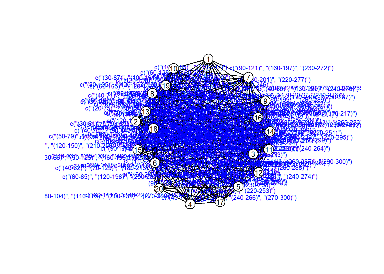
To visualize a temporal network, plotting all slices simultaneously yields a less than useful figure:
# A dataframe is read in or loaded:
  df = read.csv("./df.csv")
  n_nodes = max(c(df$tail, df$head))
  base_net = network.initialize(n_nodes, directed = FALSE)
# The dataframe should be turned into a Temporal Network:
  net_dyn = networkDynamic(
    base.net = base_net,
    edge.spells = df[, c("onset", "terminus", "tail", "head")]
  )
Created net.obs.period to describe network
Network observation period info:
Number of observation spells: 1
Maximal time range observed: 10 until 300
Temporal mode: continuous
Time unit: unknown
Suggested time increment: NA # Visualize the Temporal Network
coords = plot(net_dyn,
displaylabels=TRUE,
label.cex = 0.8,
label.pos = 5,
vertex.col = 'white',
vertex.cex = 3,
edge.label = sapply(get.edge.activity(net_dyn),function(e){
paste('(',e[,1],'-',e[,2],')',sep='')
}),
edge.label.col = 'blue',
edge.label.cex = 0.7
)
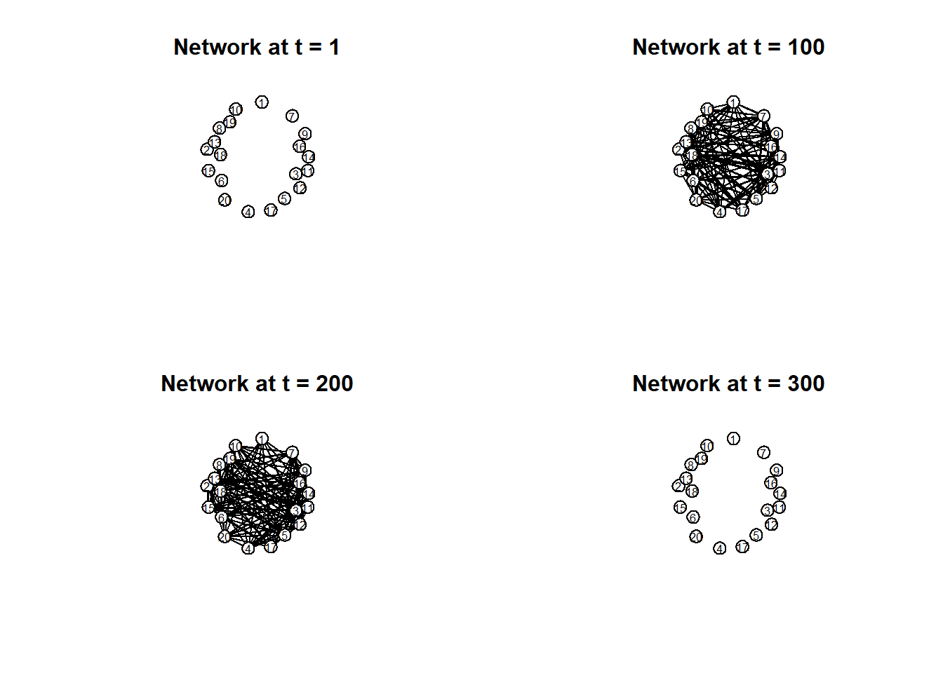
Instead, the network structure is more clearly shown by plotting separate moments in time:
# Plot separate moments in time:
  par(mfrow = c(2, 2))
  times = c(1, 100, 200, 300)
  titles = paste("Network at t =", times)
  invisible(lapply(seq_along(times), function(i) {
    plot(
      network.extract(net_dyn, at = times[i]),
      main = titles[i],
      displaylabels = TRUE,
      label.cex = 0.6,
      label.pos = 5,
      vertex.col = 'white',
      vertex.cex = 5,
      coord = coords
    )
  }))
Or have R make it for you:
filmstrip(net_dyn, frames = 4, displaylabels = FALSE)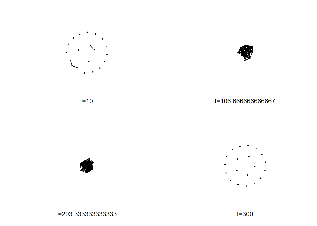
But you have no control over this. Instead, you may create a more controlled animation:
compute.animation(
    net_dyn,
    animation.mode = "kamadakawai",
    slice.par = list(
      start = 1,
      end = 310,
      interval = 10,
      aggregate.dur = 10,
      rule = "any"
    )
  )
render.d3movie(
    net_dyn,
    output.mode = "htmlWidget",
    displaylabels = FALSE,
    # This slice function makes the labels work
    vertex.tooltip = function(slice) {
      paste(
        "<b>Name:</b>", (slice %v% "name"),
        "<br>",
        "<b>Region:</b>", (slice %v% "region")
      )
    }
  )
Modeling Network Metrics through Time
Temporal Paths and Distances
Unlike static networks, transmission between nodes can only occur if the ordered time series of events links them. In other words, the existence of paths between nodes \(i\) and \(j\) and nodes \(j\) and \(k\) do not necessarily mean a path exists between nodes \(i\) and \(k\), as these events may not occur in sequence. The shortest temporal distance between nodes is thus the time difference between one node communicating to another (Thompson et al. 2017). See Thompson et al. (2017) figure 1, where information from \(node 1\) can only reach \(node 5\) through one time-respecting path, which would be different if the network were static:
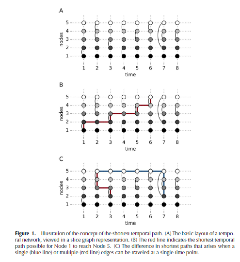
Thompson et al. (2017)
Consequently, calculation of distance between nodes (closeness) must take the network’s temporal dimension into account. Average temporal distance between nodes, defined as the average time it takes to complete time-ordered shortest paths between nodes (Pan and Saramaki 2011) measures among other things the speed of the dynamics the network is modeling. For example, in infectious disease transmission, average temporal distance might measure how quickly the disease is spreading between patients.
Come up with an example from psychology where average temporal distance might give you relevant information about your psychological temporal network.
Ideas
- Social learning (morality, social mores)
- Information propagation (emails, human memory)
Number of plot connections over time.
# Observing the number of connections as a function of time
  plot(tEdgeFormation(net_dyn, time.interval = 1))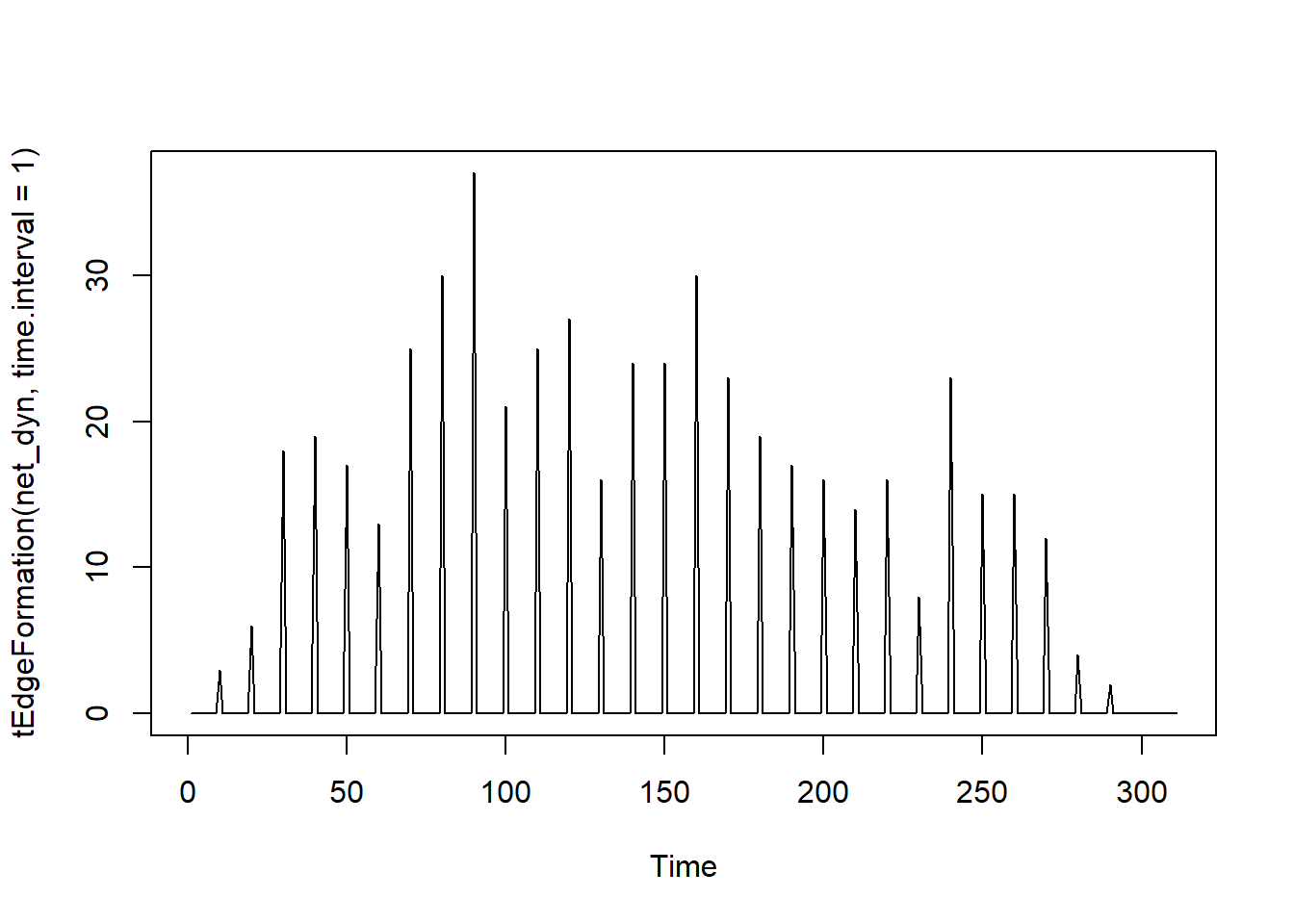
Focusing on a specific node, can also acknowledge how tracking a single path \(v^{th}\) node
v1path = tPath(net_dyn,v = 1, direction = "fwd")
  print(v1path)
$tdist
[1] 0 19 29 29 29 29 29 29 29 29 29 29 29 29 29 39 29 29 29 19
$previous
[1] 0 1 2 3 8 1 3 3 20 8 7 20 3 11 2 3 8 4 7 1
$gsteps
[1] 0 1 2 3 4 1 3 3 2 4 4 2 3 5 2 3 4 4 4 1
$start
[1] 1
$end
[1] Inf
$direction
[1] "fwd"
$type
[1] "earliest.arrive"
attr(,"class")
[1] "tPath" "list" Another measure of temporal paths includes setting a ceiling of allowed time between consecutive events, modeling events such as an infected person waiting until the infection fades before interacting with another person in a social network. Calculating the effect of this cutoff time includes calculating the proportion of node pairs connected by temporal paths within the observation period, AKA the reachability ratio (Pan & Saramaki 2011).
Holme & Saramaki 2012 refers to the reachability ratio as the “average fraction of vertices in the sets of influence of all vertices,” where the set of influence of vertex/node \(i\) is defined as the set of nodes that can be reached by time-respecting paths from node \(i\). The reachability ratio in itself can also be used as a measure of centrality or network efficiency. Changes in reachability ratio can reflect valuable information about the system modeled by the network; for example, reachability ratio might increase at a consistent time point after new information is given to a communication network, suggesting a timeframe for information dissemination (Holme & Saramaki 2012).
For more detail on reachability ratios, see this definition from Jonathan:
Reachability is essentially a centrality measure of whether a given node can eventually reach another node in the domain of [0, T].
- A node can always reach itself, so its reachability ratio is at the minimum defined to be \(1/|V|\)
- If you decide to ignore that self-loop, redefine everything mentioning \(|V|\) as \(|V| - 1\)
- If a node can reach another node in time then we can just add 1 to the set of nodes it can reach which can extend from \([1, |V|]\)
- You should then have–for each node–a value between \([1, |V|]\) which represents whether the ith node could reach any other node in the domain of time you allotted
- The reachability ratio for a given node is the proportion of \(|V|\) could node i reach through time
- The average reachability ratio could then be the mean of those ratios.
How does this idea of reachability differ from a static di-graph?
Temporal vs Static Distances
The relationship between static and temporal average distances varies depending on the network. For example, it is nonlinear in social networks (Pan and Saramaki 2011). In both static and temporal networks, the centrality measure of closeness is a measure of how quickly all other nodes can be reached from a given node (Pan & Saramaki 2011).
How does this measure of closeness differ or not from static networks? Are there benefits of thinking of closeness through a temporal vs static lens?
tdist: distance from t = origin for v to affect the \(i^{th}\) node previous: The node that immediately preceded landing on the \(i^{th}\) node gsteps: The number of “graph” steps to get to the \(i^{th}\) node
plot(v1path,
       coord = coords,
       displaylabels=TRUE)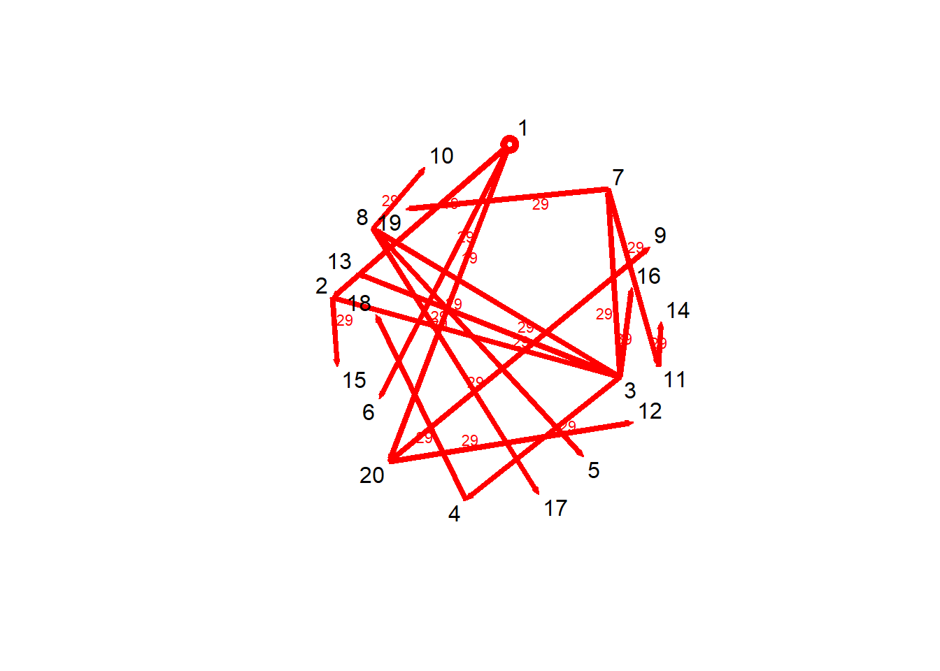
  # Plotting function from tutorial website:
    # plotPaths(
    #   net_dyn,
    #   v1path,
    #   displaylabels = FALSE,
    #   vertex.col = "white"
    # )
Other measures, such as density and degree (defined as you would for a static network, calculated per time slice), can also be visualized:
# Observing graph-based density as a function of time
  dynamicdensity = tSnaStats(
    net_dyn,
    snafun = "gden",
    start = 1,
    end = 300,
    time.interval = 1,
    aggregate.dur = 10
  )
  plot(dynamicdensity)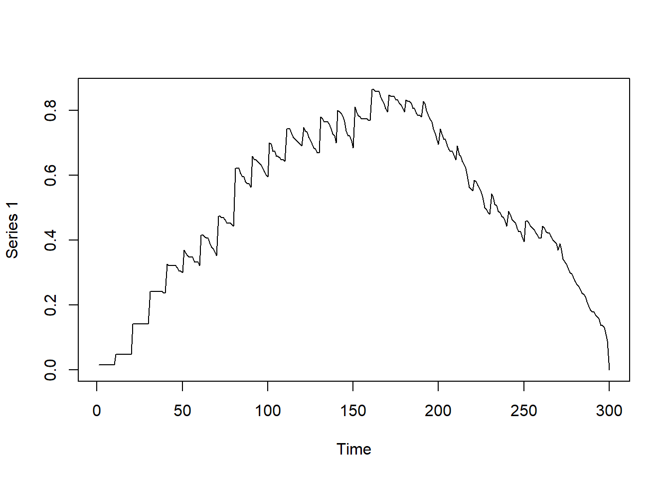
# Observing degree in the graph over time
  dynamicdeg = tSnaStats(
    net_dyn,
    snafun = "centralization",
    start = 1,
    end = 300,
    time.interval = 1,
    aggregate.dur = 10,
    FUN = "degree"
  )
  plot(dynamicdeg)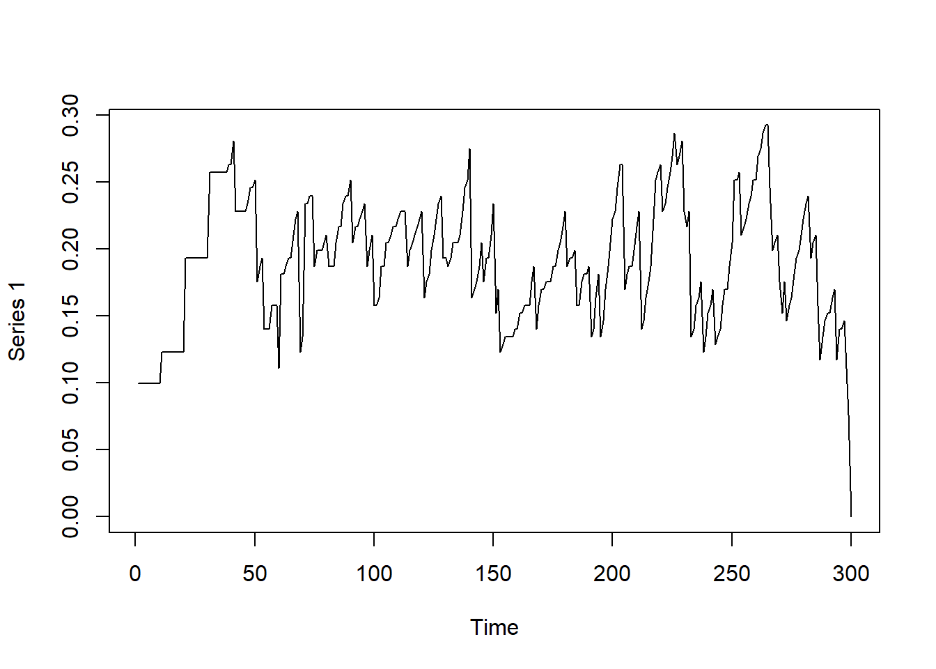
Now that you have a time series of the centrality measures of the temporal network, you may analyze the time series as you wish to following standard time series analysis procedures.
Dynamic Networks
What are dynamic networks? What are the different ways we can think of dynamic networks?
In contrast to the temporal network, a dynamic network–for this class–is considered some form of model fitted to time-series observations. The parameters of the resulting fitted model form a “dynamic network.” A dynamic network is a representation of the functional, stable connections between variables across time. Another way to think about this may be as an aggregation of the same relationships between variables at each slice of time of a temporal network.
Examples of dynamic networks: - Dyadic interactions involve multiple variables often visualized as nodes evolving over time and interacting with each other. There are various ways to model such interactions as a network as has been discussed in Gates and Liu (2016). - Modeling connectivity between Regions of Interest in fMRI data
In our readings for this week specific models showed up where each paper was trying to target one portion of the idiographic to nomothetic spectrum. In your own research, where would you fall on the nomothetic and idiographic spectrum?
#Code Load library
library(OpenMx)
OpenMx functions for automatically fitting dt- and ct-var models Proprietary by Jonathan J. Park
In the function below, you need N = 1 (single-subject) time-series data You need variable names and may optionally specify the A, Q, and R matrices They represent the dynamics, process noises, and measurement error variances, respectively The equation for a state-space model is given by: ?mxExpectationStateSpace \[State: x_{t} = A x_{t-1} + B u_{t} + q_{t}\] \[Measurement: y_{t} = C x_{t} + D u_{t} + r_{t}\] Which represent the state (dynamic) and space (measurement) equations
Starting with the measurement equation, we have our observed variable \(y_t\) which is measured with errors, so we want to dis-aggregate the measurement error \(r\) from the underlying signal \(x_t\).
In the state equation, we define the dynamics of our signal \(x_t\). The signal at time \(t\), is predicted by its state in the previous time point, \(t-1\). We allow the signal to fluctuate due to some unexplained noise in the system given by the \(q_t\). We allow covariates, \(u_t\), however for the purposes of this class we will not use any covariates, hence \(B\), \(D\) are 0.
All dynamic networks in this week can be described by this formulation. The mx.var() function assumes that C is a diagonal matrix R is diagonal and ~0.00 (i.e., assumes no measurement error) Q is assumed diagonal with variances = 1.00 B is 0 for this demonstration because there will be no covariates in either the state or measurement equation level. All can be changed by user-specification.
The point of this code is to define the matrices in the state and measurement equations discussed above.
 mx.var = function(dataframe = NULL, varnames = paste0('y', 1:nvar),
                    Amat = NULL, Qmat = NULL, Rmat = NULL){
    ne = length(varnames)
    ini.cond = rep(0, ne)
    if(is.null(Amat)){
      Amat = matrix(0, ne, ne)
    }
    if(is.null(Qmat)){
      Qmat = diag(1, ne)
    }
    if(is.null(Rmat)){
      Rmat = diag(1e-5, ne)
    }
    amat = mxMatrix('Full', ne, ne, TRUE, Amat, name = 'A')
    bmat = mxMatrix('Zero', ne, ne, name='B')
    cdim = list(varnames, paste0('F', 1:ne))
    cmat = mxMatrix('Diag', ne, ne, FALSE, 1, name = 'C', dimnames = cdim)
    dmat = mxMatrix('Zero', ne, ne, name='D')
    qmat = mxMatrix('Symm', ne, ne, FALSE, diag(ne), name='Q', lbound=0)
    rmat = mxMatrix('Symm', ne, ne, FALSE, diag(1e-5, ne), name='R')
    xmat = mxMatrix('Full', ne, 1, FALSE, ini.cond, name='x0', lbound=-10, ubound=10)
    pmat = mxMatrix('Diag', ne, ne, FALSE, 1, name='P0')
    umat = mxMatrix('Zero', ne, 1, name='u')
    osc = mxModel("OUMod", amat, bmat, cmat, dmat, qmat, rmat, xmat, pmat, umat,
                  mxExpectationStateSpace('A', 'B', 'C', 'D', 'Q',
                                          'R', 'x0', 'P0', 'u'),
                  mxFitFunctionML(), mxData(dataframe, 'raw'))
    oscr = mxTryHard(osc)
    return(ModRes = oscr)
 }
Auto-Regressive (1) Model
Let’s start simple with a univariate state space model.
What is an autoregression?
The autoregression of a variable essentially describes its inertia, or how similar/dissimilar it is to itself over time. Regressing a variable at a specific time point to itself in the previous time point provides a beta coefficient which would be called the autoregressive coefficient.
ne = 1
  amat = mxMatrix('Full', ne, ne, TRUE, 0.80, name = 'A')
  bmat = mxMatrix('Zero', ne, ne, name='B')
  cdim = list("AR1", paste0('F', 1:ne))
  cmat = mxMatrix('Diag', ne, ne, FALSE, 1, name = 'C', dimnames = cdim)
  dmat = mxMatrix('Zero', ne, ne, name='D')
  qmat = mxMatrix('Symm', ne, ne, FALSE, diag(ne), name='Q', lbound=0)
  rmat = mxMatrix('Symm', ne, ne, FALSE, diag(1e-5, ne), name='R')
  xmat = mxMatrix('Full', ne, 1, FALSE, 0, name='x0', lbound=-10, ubound=10)
  pmat = mxMatrix('Diag', ne, ne, FALSE, 1, name='P0')
  umat = mxMatrix('Zero', ne, 1, name='u')
  osc = mxModel("OUMod", amat, bmat, cmat, dmat, qmat, rmat, xmat, pmat, umat,
                mxExpectationStateSpace('A', 'B', 'C', 'D', 'Q',
                                        'R', 'x0', 'P0', 'u'))
  sim.data = mxGenerateData(osc, nrows = 1000)
  head(sim.data)
AR1
1 -0.002832068
2 1.256710079
3 2.336681888
4 2.746121370
5 2.756308847
6 0.164417983 plot(x = (1:nrow(sim.data)), y = sim.data$AR1, type = "l",
main = "Time-Series of AR1", ylab = "Values", xlab = "Time")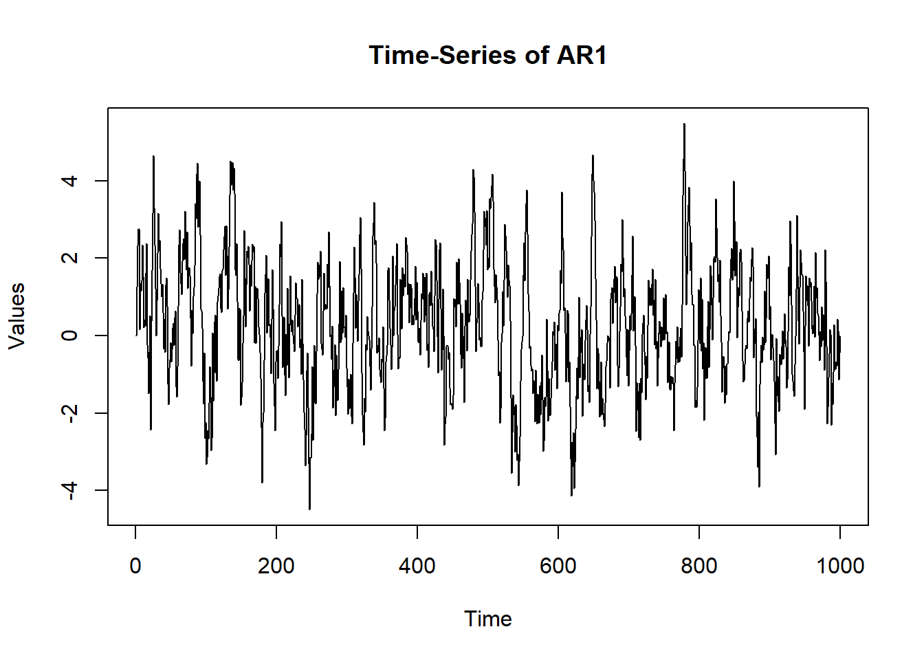
ar1 = mx.var(dataframe = sim.data, varnames = "AR1") summary(ar1)$parameters name matrix row col Estimate Std.Error lbound ubound lboundMet
1 OUMod.A[1,1] A 1 1 0.7926252 0.01946511 NA NA FALSE
uboundMet
1 FALSEExplanation of the AR(1) code:
\(ne\) stands for the number of variables which in this case is 1. The \(A\) matrix is the drift matrix which will contain the autoregressive lag-1 coefficient. The process noise variance \(q_t\) will be in the \(qmat\) and the measurement error variance \(r_t\) will be in the \(rmat\). The factor loading matrix \(cmat\) is set to 1 because we have one state that loads on only one measured variable.
We can now compare this to a different autoregressive coefficient to observe how different the two time series look and also to compare recovery of the parameter estimate:
osc$A$values = -0.80
sim.data = mxGenerateData(osc, nrows = 1000)
  plot(x = (1:nrow(sim.data)), y = sim.data$AR1, type = "l",
       main = "Time-Series of AR1", ylab = "Values", xlab = "Time")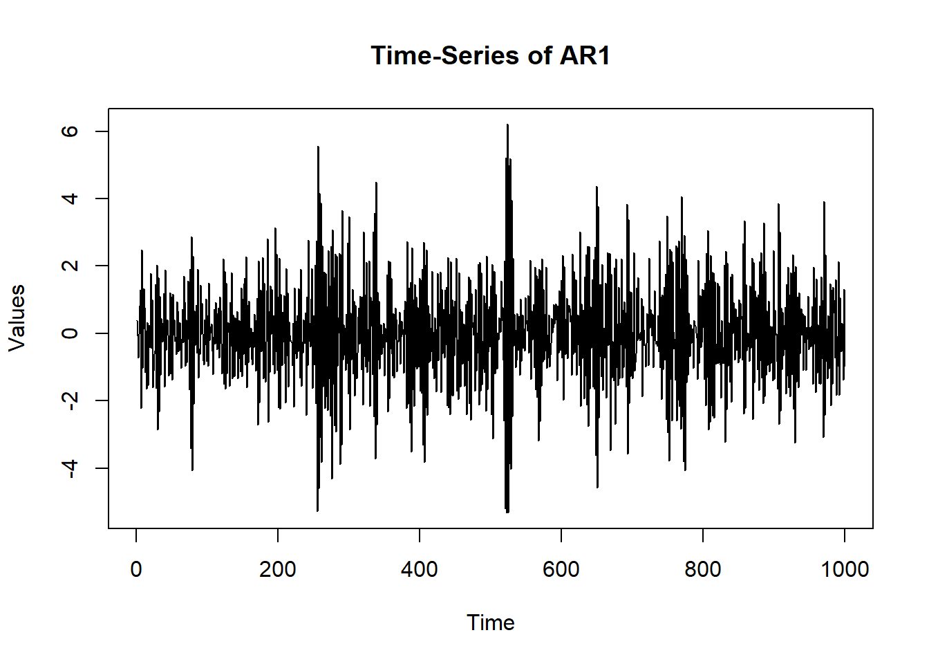
ar1 = mx.var(dataframe = sim.data, varnames = "AR1") summary(ar1)$parameters name matrix row col Estimate Std.Error lbound ubound lboundMet
1 OUMod.A[1,1] A 1 1 -0.800257 0.01954971 NA NA FALSE
uboundMet
1 FALSEWhat does a positive/ negative autoregression mean? Where can you see them?
A positive autoregression may mean that the value of my happiness score at the next time point goes up if it is going up already. A negative value of the autoregression would mean that an increase in my happiness score would mean that I will not be very happy at the very next time point. You may also think of a positive autoregression to come from a stable system while a negative value would come from an unstable one. Examples of a positive autoregression in psychology may be fluid reasoning and negative autoregression may be mood swings of a person suffering from borderline personality disorder.
VAR(1)
This is the same as AR(1) but now we have three variables instead of one. Now our drift matrix, \(A\) is 3x3 and is defined to be: \[ \underset{3\times 3}{\mathbf{A}} = \begin{bmatrix} 0.60 & 0.00 & 0.00 \\ 0.00 & 0.60 & -0.25 \\ 0.25 & 0.00 & 0.60 \end{bmatrix} \] All other matrix definitions should be similar to how we defined them in the AR(1) case.
ne = 3
  VAR.params = matrix(c(0.60, 0.00, 0.00,
                        0.00, 0.60, -0.25,
                        0.25, 0.00, 0.60), ne, ne)
  amat = mxMatrix('Full', ne, ne, TRUE, VAR.params, name = 'A')
  bmat = mxMatrix('Zero', ne, ne, name='B')
  cdim = list(paste0("V", 1:ne), paste0('F', 1:ne))
  cmat = mxMatrix('Diag', ne, ne, FALSE, 1, name = 'C', dimnames = cdim)
  dmat = mxMatrix('Zero', ne, ne, name='D')
  qmat = mxMatrix('Symm', ne, ne, FALSE, diag(ne), name='Q', lbound=0)
  rmat = mxMatrix('Symm', ne, ne, FALSE, diag(1e-5, ne), name='R')
  xmat = mxMatrix('Full', ne, 1, FALSE, 0, name='x0', lbound=-10, ubound=10)
  pmat = mxMatrix('Diag', ne, ne, FALSE, 1, name='P0')
  umat = mxMatrix('Zero', ne, 1, name='u')
  osc = mxModel("OUMod", amat, bmat, cmat, dmat, qmat, rmat, xmat, pmat, umat,
                mxExpectationStateSpace('A', 'B', 'C', 'D', 'Q',
                                        'R', 'x0', 'P0', 'u'))
  sim.data = mxGenerateData(osc, nrows = 1000)
  head(sim.data)
V1 V2 V3
1 -0.2628170 -0.52574478 0.7298529
2 -0.2229628 0.45081689 0.2990795
3 -1.9228300 -0.69924868 -1.5720479
4 -1.4678509 0.02191713 -0.4153465
5 -2.2816987 -1.73312961 -1.5554113
6 -0.8506020 -0.08621230 -0.1525898 VAR1 = mx.var(dataframe = sim.data, varnames = paste0("V", 1:ne)) summary(VAR1)$parameters name matrix row col Estimate Std.Error lbound ubound lboundMet
1 OUMod.A[1,1] A 1 1 0.601967332 0.02231789 NA NA FALSE
2 OUMod.A[2,1] A 2 1 0.014061008 0.02231728 NA NA FALSE
3 OUMod.A[3,1] A 3 1 -0.004919610 0.02231811 NA NA FALSE
4 OUMod.A[1,2] A 1 2 0.031442705 0.02594573 NA NA FALSE
5 OUMod.A[2,2] A 2 2 0.552466835 0.02594743 NA NA FALSE
6 OUMod.A[3,2] A 3 2 -0.251149409 0.02594755 NA NA FALSE
7 OUMod.A[1,3] A 1 3 0.255622652 0.02370838 NA NA FALSE
8 OUMod.A[2,3] A 2 3 0.001340486 0.02370865 NA NA FALSE
9 OUMod.A[3,3] A 3 3 0.632859157 0.02370966 NA NA FALSE
uboundMet
1 FALSE
2 FALSE
3 FALSE
4 FALSE
5 FALSE
6 FALSE
7 FALSE
8 FALSE
9 FALSE params = matrix(0, ne, ne)
for(i in 1:nrow(summary(VAR1)$parameters)){
params[summary(VAR1)$parameters[i,"row"], summary(VAR1)$parameters[i, "col"]] =
ifelse(abs(summary(VAR1)$parameters[i,"Estimate"]) > qnorm(0.975) * summary(VAR1)$parameters[i,"Std.Error"],
summary(VAR1)$parameters[i,"Estimate"],
0.00)
}We set the values that were not significant in the drift matrix to 0.00 and print it here. In practice, we would use this pruned params matrix as an initial value of the drift matrix when we begin the estimation procedure again. We do not do it here for the sake of brevity.
# True
    VAR.params
[,1] [,2] [,3]
[1,] 0.6 0.00 0.25
[2,] 0.0 0.60 0.00
[3,] 0.0 -0.25 0.60 # Estimated
round(params, 2) [,1] [,2] [,3]
[1,] 0.6 0.00 0.26
[2,] 0.0 0.55 0.00
[3,] 0.0 -0.25 0.63Graphical VAR
Now that we are experts in VAR(1), let’s fit this data to a graphical VAR. The GVAR gives us the same temporal network as a VAR would, but it also gives us a contemporaneous network.
What are contemporaneous networks?
As defined by Gates and Liu (2016), contemporaneous “effects indicate the extent to which values of another variable instantaneously relate to a given variable after controlling for lagged effects (but variables are not allowed to predict themselves contemporaneously).”
Why do we care about contemporaneous networks?
One possible reason
Play behavior in same-sex dyads When coded at intervals of 10 seconds, Beltz et al. (2013) found that girls’ levels of positive affect were dependent on their peers’ prior positive affect more so than boys’, whereas for boys, the current level of vigor in activity was predicted by their peers’ current levels of activity.
library(graphicalVAR)
gvar <- graphicalVAR(sim.data, verbose = FALSE)
summary(gvar)
=== graphicalVAR results ===
Number of nodes: 3
Number of tuning parameters tested: 2500
EBIC hyperparameter: 0.5
Optimal EBIC: 1329.919
Number of non-zero Partial Contemporaneous Correlations (PCC): 0
PCC Sparsity: 1
Number of PCC tuning parameters tested: 50
PCC network stored in object$PCC
Number of non-zero Partial Directed Correlations (PDC): 1
PDC Sparsity: 0.6666667
Number of PDC tuning parameters tested: 50
PDC network stored in object$PDC
Use plot(object) to plot the estimated networks.plot(gvar)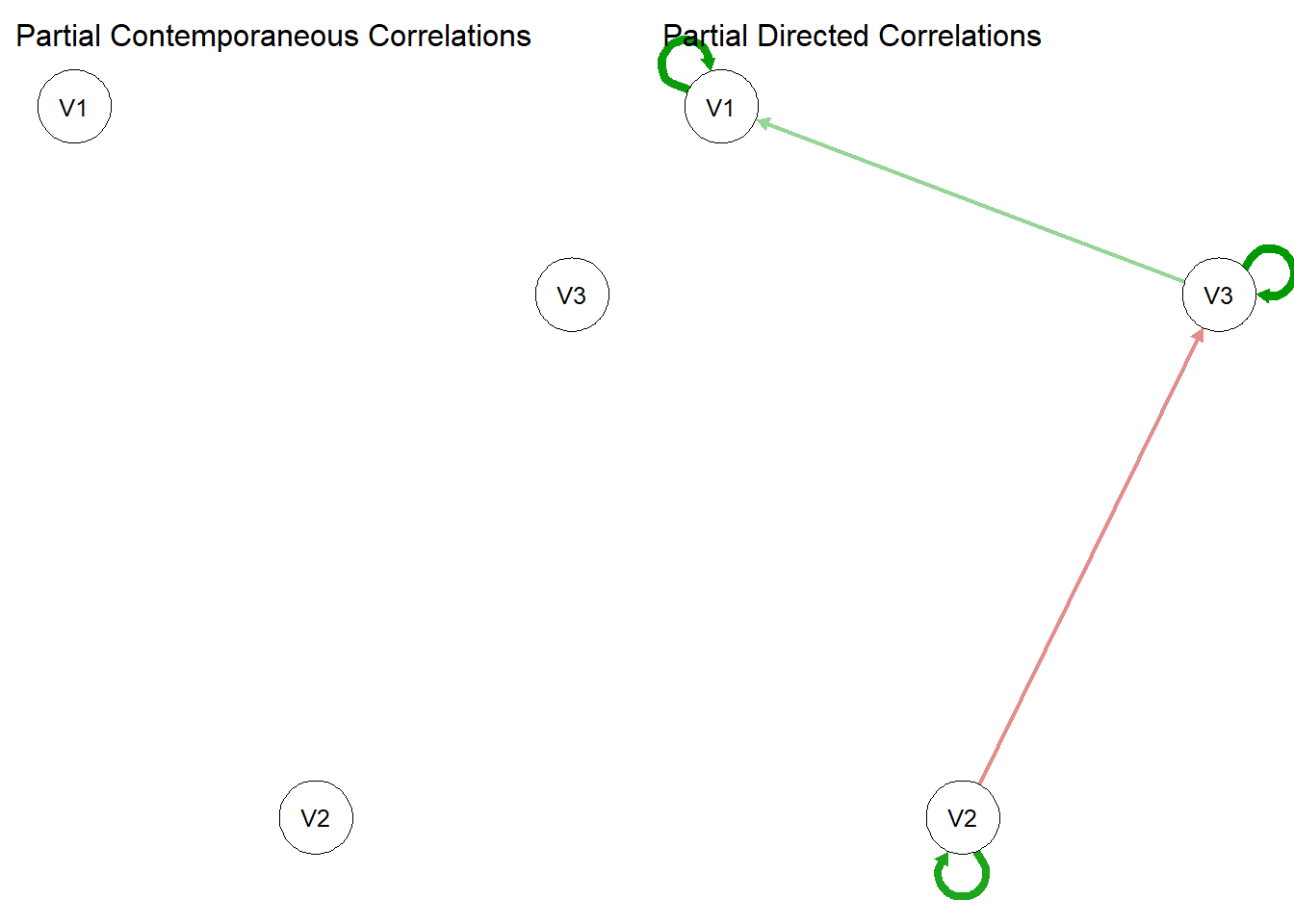
Why is the contemporaneous network empty?
Hmmmmm………….
We initially simulated the VAR(1) model with \(Q = I\) which means the off-diagonal elements were constrained to be zero. Hence there were no edges in the contemporaneous network.
  Q <- matrix(c(1,.7, 0,.7,1,0,0,0,1), 3,3)
  osc$Q$values = Q
  sim.data = mxGenerateData(osc, nrows = 1000)

gvar2 <- graphicalVAR(sim.data, verbose = FALSE)
summary(gvar2)
=== graphicalVAR results ===
Number of nodes: 3
Number of tuning parameters tested: 2500
EBIC hyperparameter: 0.5
Optimal EBIC: 811.9997
Number of non-zero Partial Contemporaneous Correlations (PCC): 1
PCC Sparsity: 0.6666667
Number of PCC tuning parameters tested: 50
PCC network stored in object$PCC
Number of non-zero Partial Directed Correlations (PDC): 1
PDC Sparsity: 0.6666667
Number of PDC tuning parameters tested: 50
PDC network stored in object$PDC
Use plot(object) to plot the estimated networks.plot(gvar2) 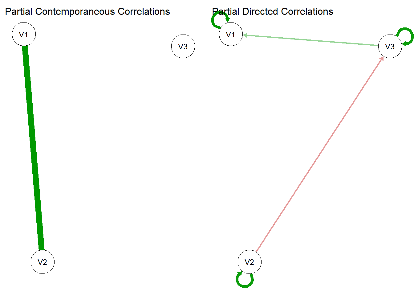
BEAUTIFUL! Now, when we simulated the data with \(Q[2,1] = Q[1,2] = 0.7\) we made the V1 to V2 edge show up in the contemporaneous network.
Continuous Time - AR
Now we move to continuous AR, pretending as if discrete time AR was not difficult enough. This follows the same state space framework as before so you will find the code to be essentially the same. The only difference would be in how the parameters are estimated, so we use mxExpectationSSCT instead of mxExpectationSS. Also we set the discrete time lag 1 autoregressive coefficient to 0.6 to simulate the data.
  mx.ctvar = function(dataframe = NULL, varnames = paste0('y', 1:nvar),
                      Amat = NULL, Qmat = NULL, Rmat = NULL){
    ne = length(varnames)
    ini.cond = rep(0, ne)
    if(is.null(Amat)){
      Amat = matrix(0, ne, ne)
    }
    if(is.null(Qmat)){
      Qmat = diag(1, ne)
    }
    if(is.null(Rmat)){
      Rmat = diag(1e-5, ne)
    }
    amat = mxMatrix('Full', ne, ne, TRUE, Amat, name = 'A')
    bmat = mxMatrix('Zero', ne, ne, name='B')
    cdim = list(varnames, paste0('F', 1:ne))
    cmat = mxMatrix('Diag', ne, ne, FALSE, 1, name = 'C', dimnames = cdim)
    dmat = mxMatrix('Zero', ne, ne, name='D')
    qmat = mxMatrix('Symm', ne, ne, FALSE, diag(ne), name='Q', lbound=0)
    rmat = mxMatrix('Symm', ne, ne, FALSE, diag(1e-5, ne), name='R')
    xmat = mxMatrix('Full', ne, 1, FALSE, ini.cond, name='x0', lbound=-10, ubound=10)
    pmat = mxMatrix('Diag', ne, ne, FALSE, 1, name='P0')
    umat = mxMatrix('Zero', ne, 1, name='u')
    tmat = mxMatrix('Full', 1, 1, FALSE, name='time', labels='data.Time')

    osc = mxModel("OUMod", amat, bmat, cmat, dmat, qmat, rmat, xmat, pmat, umat, tmat,
                  mxExpectationSSCT('A', 'B', 'C', 'D', 'Q',
                                    'R', 'x0', 'P0', 'u', 'time'),
                  mxFitFunctionML(), mxData(dataframe, 'raw'))
    oscr = mxTryHard(osc)
    return(ModRes = oscr)
  }

  ne = 1
  amat = mxMatrix('Full', ne, ne, TRUE, 0.60, name = 'A')
  bmat = mxMatrix('Zero', ne, ne, name='B')
  cdim = list("AR1", paste0('F', 1:ne))
  cmat = mxMatrix('Diag', ne, ne, FALSE, 1, name = 'C', dimnames = cdim)
  dmat = mxMatrix('Zero', ne, ne, name='D')
  qmat = mxMatrix('Symm', ne, ne, FALSE, diag(ne), name='Q', lbound=0)
  rmat = mxMatrix('Symm', ne, ne, FALSE, diag(1e-5, ne), name='R')
  xmat = mxMatrix('Full', ne, 1, FALSE, 0, name='x0', lbound=-10, ubound=10)
  pmat = mxMatrix('Diag', ne, ne, FALSE, 1, name='P0')
  umat = mxMatrix('Zero', ne, 1, name='u')
  osc = mxModel("OUMod", amat, bmat, cmat, dmat, qmat, rmat, xmat, pmat, umat,
                mxExpectationStateSpace('A', 'B', 'C', 'D', 'Q',
                                        'R', 'x0', 'P0', 'u'))
  sim.data = mxGenerateData(osc, nrows = 1000)
  sim.data$Time = 0:(nrow(sim.data)-1)
ct.ar = mx.ctvar(dataframe = sim.data, varnames = "AR1") summary(ct.ar)Summary of OUMod
free parameters:
name matrix row col Estimate Std.Error A
1 OUMod.A[1,1] A 1 1 -0.341768 0.02662509
Model Statistics:
| Parameters | Degrees of Freedom | Fit (-2lnL units)
Model: 1 999 2953.988
Saturated: 2 998 NA
Independence: 2 998 NA
Number of observations/statistics: 1000/1000
Information Criteria:
| df Penalty | Parameters Penalty | Sample-Size Adjusted
AIC: 955.988 2955.988 2955.992
BIC: -3946.859 2960.896 2957.720
To get additional fit indices, see help(mxRefModels)
timestamp: 2025-06-03 23:04:03
Wall clock time: 0.1069388 secs
optimizer: SLSQP
OpenMx version number: 2.21.13
Need help? See help(mxSummary) WOAH?! Why is the estimate off by such a huge margin? Maybe they aren’t stable yet. Let’s use these values to refit the model.
ct.ar2 = mx.ctvar(dataframe = sim.data, varnames = "AR1", A = -.35) summary(ct.ar2)Summary of OUMod
free parameters:
name matrix row col Estimate Std.Error A
1 OUMod.A[1,1] A 1 1 -0.3417679 0.02662506
Model Statistics:
| Parameters | Degrees of Freedom | Fit (-2lnL units)
Model: 1 999 2953.988
Saturated: 2 998 NA
Independence: 2 998 NA
Number of observations/statistics: 1000/1000
Information Criteria:
| df Penalty | Parameters Penalty | Sample-Size Adjusted
AIC: 955.988 2955.988 2955.992
BIC: -3946.859 2960.896 2957.720
To get additional fit indices, see help(mxRefModels)
timestamp: 2025-06-03 23:04:03
Wall clock time: 0.07192397 secs
optimizer: SLSQP
OpenMx version number: 2.21.13
Need help? See help(mxSummary) Still the same! What’s going on?
Explanation:
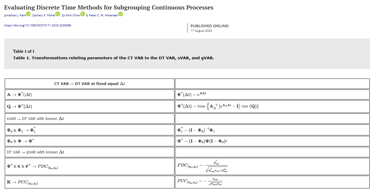
Look at the Drift matrix transformation. To convert the continuous time autoregressive coefficient to its discrete time counterpart: \(a_{dt} = e^{a_{ct}*\delta t}\)
\(a_{dt}\) is the autoregressive coefficient for the discrete time model while \(a_{ct}\) is the continuous time counterpart. \(\delta t\) is the time interval of measurement. Say you measure mood using daily diary measures then your \(\delta t\) is 1 whereas if you measure them weekly then \(\delta t = 7\). The time interval at which you study psychological processes may have an effect on your parameter estimates (Park et al., 2024).
# Identifying the discrete-time AR(1) given the CT-AR estimate by:
    # expm(a_{1,1} * Delta_t)
    expm(matrix(summary(ct.ar)$parameters$Estimate, 1, 1) * 1.00)
[,1]
[1,] 0.710513 # Compared to True Value:
0.60[1] 0.6Close (?) Is anyone interested in seeing why the transformation is exactly this? We would need to use some Ordinary Differential Equation solutions for that…
CT-VAR
Now we move to continuous time VAR(1) with three variables. Again this is very similar to its discrete time counterpart. The code stays the same in most parts.
  ne = 3
  VAR.params = matrix(c(0.60, 0.00, 0.00,
                        0.00, 0.60, -0.25,
                        0.25, 0.00, 0.60), ne, ne)
  amat = mxMatrix('Full', ne, ne, TRUE, VAR.params, name = 'A')
  bmat = mxMatrix('Zero', ne, ne, name='B')
  cdim = list(paste0("V", 1:ne), paste0('F', 1:ne))
  cmat = mxMatrix('Diag', ne, ne, FALSE, 1, name = 'C', dimnames = cdim)
  dmat = mxMatrix('Zero', ne, ne, name='D')
  qmat = mxMatrix('Symm', ne, ne, FALSE, diag(ne), name='Q', lbound=0)
  rmat = mxMatrix('Symm', ne, ne, FALSE, diag(1e-5, ne), name='R')
  xmat = mxMatrix('Full', ne, 1, FALSE, 0, name='x0', lbound=-10, ubound=10)
  pmat = mxMatrix('Diag', ne, ne, FALSE, 1, name='P0')
  umat = mxMatrix('Zero', ne, 1, name='u')
  osc = mxModel("OUMod", amat, bmat, cmat, dmat, qmat, rmat, xmat, pmat, umat,
                mxExpectationStateSpace('A', 'B', 'C', 'D', 'Q',
                                        'R', 'x0', 'P0', 'u'))
  sim.data = mxGenerateData(osc, nrows = 1000)
  sim.data$Time = 0:(nrow(sim.data)-1)
ct.var = mx.ctvar(dataframe = sim.data, varnames = paste0("V", 1:ne)) summary(ct.var)Summary of OUMod
free parameters:
name matrix row col Estimate Std.Error A
1 OUMod.A[1,1] A 1 1 -0.27932521 0.02197521
2 OUMod.A[2,1] A 2 1 -0.06577910 0.02505475
3 OUMod.A[3,1] A 3 1 -0.12826706 0.02451562
4 OUMod.A[1,2] A 1 2 0.10257389 0.03299379
5 OUMod.A[2,2] A 2 2 -0.33619210 0.02957285
6 OUMod.A[3,2] A 3 2 -0.30893496 0.03367767
7 OUMod.A[1,3] A 1 3 0.29686877 0.02935515
8 OUMod.A[2,3] A 2 3 0.08217844 0.03024809
9 OUMod.A[3,3] A 3 3 -0.33503549 0.02668422
Model Statistics:
| Parameters | Degrees of Freedom | Fit (-2lnL units)
Model: 9 2991 8676.942
Saturated: 9 2991 NA
Independence: 6 2994 NA
Number of observations/statistics: 1000/3000
Information Criteria:
| df Penalty | Parameters Penalty | Sample-Size Adjusted
AIC: 2694.942 8694.942 8695.124
BIC: -11984.154 8739.112 8710.528
CFI: NA
TLI: 1 (also known as NNFI)
RMSEA: 0 [95% CI (NA, NA)]
Prob(RMSEA <= 0.05): NA
To get additional fit indices, see help(mxRefModels)
timestamp: 2025-06-03 23:04:07
Wall clock time: 2.891986 secs
optimizer: SLSQP
OpenMx version number: 2.21.13
Need help? See help(mxSummary) params = matrix(0, ne, ne)
for(i in 1:nrow(summary(ct.var)$parameters)){
params[summary(ct.var)$parameters[i,"row"], summary(ct.var)$parameters[i, "col"]] =
ifelse(abs(summary(ct.var)$parameters[i,"Estimate"]) > qnorm(0.975) * summary(ct.var)$parameters[i,"Std.Error"],
summary(ct.var)$parameters[i,"Estimate"],
0.00)
}
params [,1] [,2] [,3]
[1,] -0.2793252 0.1025739 0.29686877
[2,] -0.0657791 -0.3361921 0.08217844
[3,] -0.1282671 -0.3089350 -0.33503549These are the parameter estimates after we drop the insignificant values in the drift matrix. We then use the same matrix as an initial value of the drift matrix when we try to re-estimate the CTVAR to ensure stability of our estimates.
ct.var2 = mx.ctvar(dataframe = sim.data, varnames = paste0("V", 1:ne), Amat = params)summary(ct.var2)$parameters name matrix row col Estimate Std.Error lbound ubound lboundMet
1 OUMod.A[1,1] A 1 1 -0.27932520 0.02197410 NA NA FALSE
2 OUMod.A[2,1] A 2 1 -0.06577910 0.02505235 NA NA FALSE
3 OUMod.A[3,1] A 3 1 -0.12826707 0.02451443 NA NA FALSE
4 OUMod.A[1,2] A 1 2 0.10257389 0.03299212 NA NA FALSE
5 OUMod.A[2,2] A 2 2 -0.33619211 0.02957053 NA NA FALSE
6 OUMod.A[3,2] A 3 2 -0.30893496 0.03367509 NA NA FALSE
7 OUMod.A[1,3] A 1 3 0.29686877 0.02935394 NA NA FALSE
8 OUMod.A[2,3] A 2 3 0.08217844 0.03024426 NA NA FALSE
9 OUMod.A[3,3] A 3 3 -0.33503549 0.02668190 NA NA FALSE
uboundMet
1 FALSE
2 FALSE
3 FALSE
4 FALSE
5 FALSE
6 FALSE
7 FALSE
8 FALSE
9 FALSECompare recovery by converting the continuous time drift matrix to its discrete time counterpart.
#discrete values
    expm(matrix(summary(ct.var2)$parameters$Estimate, 3,3) * 1.00)
[,1] [,2] [,3]
[1,] 0.74035440 0.04133733 0.21894449
[2,] -0.05162636 0.70361894 0.05099806
[3,] -0.08592006 -0.22306904 0.69308944#true
VAR.params [,1] [,2] [,3]
[1,] 0.6 0.00 0.25
[2,] 0.0 0.60 0.00
[3,] 0.0 -0.25 0.60QnA
After all of this discussion, how would you use temporal and dynamic networks in your own work? If they are not directly applicable to your research questions, could you try to think of other topics in your field where they might apply?
What may be some potentials drawbacks of these temporal and dynamic networks? Potential solutions?
Hint
The dynamic models update all the variables at the same time step, ie, synchronous updating. Maybe we have variables that operate in very different time scales and we want to incorporate that in our models.
Solution: Move to Boolean networks. More next week…..