if(!require("igraph")) install.packages("igraph")
if(!require("stats")) install.packages("stats")
if(!require("mclust")) install.packages("mclust")
if(!require("ppclust")) install.packages("ppclust")
# adjacency.matrix = readRDS("AdjMat1.RDS")
adjacency.matrix = readRDS("AdjMat2.RDS")PSC-290: Community Detection
Overview
For this section, we will be considering, what is community detection? and how can we identify communities computationally?.
First, how would you define a “community”?
Think a little before clicking.
Below are a small handful of definitions from this week’s readings:
- “A community is a subgraph of a network whose nodes are more tightly connected with each other than nodes outside the subgraph” (Fortunato & Barthélemy, 2007, p. 6)1
- “Dense subgraphs of sparse graphs (Pons & Latapy, 2006, p. 191)2
- “Homogeneity within a cluster and heterogeneity between clusters” (Steinley, 2006)3
Synonymous terms could include: modules, clusters, partitions, subgraphs.
Goals
Given communities can exist in a variety of data structures, this presents us with a few different challenges and goals:
- How to estimate the boundaries of communities within a network via computers.
- How to assess the accuracy of detected communities.
- Identify areas of opportunity for refining traditional metrics and algorithms used in community detection.
Readings Review
With these goals in mind, let’s discuss key takeaways and thoughts from this past week’s readings.
- What other goals of community detection, or what needs can it meet?
- Were there lingering questions or concern after reading them?
Psychological Relevance
Based on your area of study or personal experience, consider the following:
What are some examples of networks where you would imagine communities existing?
Is community detection, modularity, or cluster identification a challenge in your area of study? How so?
under which conditions these community detections can be easily misleading?
Approaches
For this next section, we will be covering a spread of approaches that can be used to detect communities in networks.
We will use the following packages and data:
k-means Clustering
Steinley, 2006
- innumerable ways to partition a network
- homogeneity WITHIN a cluster and heterogeneity BETWEEN clusters
in plain words: To divide data points into k-groups (clusters) such that points in the same cluster are more similar to each other than to those in other clusters.
k-means Clustering: a discrete community detection algorithm that aim to minimize within-cluster variance
Objective function (Park et al., 2024) [^park]
\[J(X) = \sum_{j=1}^C \sum_{i=1}^{n_j} \Vert \mathbf{x}_i - \bar{\mathbf{x}}_j \Vert^2\] C: total number of communities to partition j: cluster index
\[\Vert \mathbf{x}_i - \bar{\mathbf{x}}_j \Vert^2\] The squared Euclidean distance between a point Xi and its custer center.
\[inner sum = \sum_{i=1}^{n_j} \Vert \mathbf{x}_i - \bar{\mathbf{x}}_j \Vert^2\] the total squared distance of all points in cluster j to the cluster center
\[outer sum = \sum_{j=1}^C\] adds these distances across all C clusters, and C is pre-specified.
Basically, this algorithm partitions dataset into C non-overlapping clusters.
method
Plain words
pre-specify K
Initialize K cluster centroids
Assign each data point to the nearest centroid using the Euclidean distance
update centroids -repeat until convergence
\(N \times P\) into \(K\) classes (\(C_1, C_2, ..., C_K)\), where \(N\) = objects with measurements on \(P\) variables (Steinley, 2006, p. 2); this page has a generally good set of formulas and notation to include under section 2
centroids (cluster center) and K is predetermined
starting values matter! discuss initialization (p. 6, section 3.2)
- random partitions based on \(K\) classes as starting values
- ‘rational’ starts -> “subject matter expertise” BUT K should be varied (so a less common approach)
determining K: aKa the “correct” number of clusters
- NO hierarchical clustering (p. 7)
- three methods: algorithmic, graphical, formulaic
- algorithmic: \(\psi\) = refining parameter
3.4: variables to use
- variable standardization: standardization by the range?
- variable selection + weighting
4: theoretical results
- evaluating clusters, 4.2.2
n.nodes.per.group <- 10 # each custer is assumped to have 10 nodes
n.groups <- 5 #Five groups

results.1 = lapply(1:round(((n.nodes.per.group*n.groups)/5)), # generating a range of potential k-values (1:10)
                   function(k) kmeans(adjacency.matrix, # applying the k-means function to the above range
                                      centers = k,
                                      iter.max = 1000,
                                      nstart = 30)) #run k-means 30 times with different random initializations and picks the lowest within-cluster sum of squares
wss.vals = sapply(results.1, function(res) sum(res$withinss)) # extracting WSS
plot(wss.vals, type = "l") # plotting the within-cluster variance 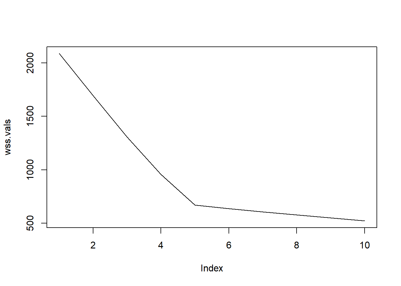
- What is the purpose of this code?
- Try different numbers of clusters (K) on an adjacency matrix
- Run K-means for each K
- Compute the WSS each
- plot the WSS
This provide WSS plot for K=1 to 10 where is the optimal number of clusters?
No chance of overlappig -> Fuzzy C-Means
Here is link to an interactive visualization demonstrating k-means clustering
Reflection Question
Which research questions (in psychological field) can use this algorithm (no chance for overlap)?
Fuzzy c-Means Clustering
Park, Chow, & Molenaar, 2024
- a direct extension of k-means
- related concept, bridges, but still maintains distinct groups
- “likelihood of membership for subjects across multiple groups”
- “fuzzifier”: no distributional assumptions
Rather than discretely categorizing, a fuzzy cluster provides likelihood that each data point (individuals) belong to Group A and Group B (saperately)
Fuzzy community detection is a method used to group individuals (or items) into overlapping communities Instead of saying this data point (individual) belong to Group A, Fuzzy methods say this data point (individual) might be 60% in Group A and 40% group B.
real-life data isn’t always clear-cut
Objective Function:
\[ J(U, X) = \sum_{j=1}^{C}\sum_{i=1}^{N} \mu_{ij}^m \Vert \mathbf{x}_i - \bar{\mathbf{x}_j} \Vert^2\]
N: Number of data points C: number of clusters j: cluster index \[\mu_{ij}^m\] membership degree of point i in cluster j m: fuzziness parameter (larger m, fuzzier cluster)
\[\mu_{ij}^m = \frac{1}{\sum_{k=1}^{C} (\frac{\Vert \mathbf{x}_i - \bar{\mathbf{x}_j} \Vert}{\Vert \mathbf{x}_i - \bar{\mathbf{x}_k} \Vert})^{\frac{2}{m-1}}}\] a membership degree: “a membership degree closer to 1 then indicates that a subject is closer -…-to be a member of an assigned community relative to another (park et al.,2024)
- Initialize membership matrix U
randomly assign a degree of membership
- Compute Centroids (as a weighted average)
so, a cluster center would be more pulled towards the point that belong to it more confidently
Update membership matrix U
Repeat until convergence
# running Fuzzy C-means clustering for different value of k (number of cluster from 1 to 25)
results.2 = lapply(1:round(((n.nodes.per.group*n.groups))/2),
                   function(k) fcm(adjacency.matrix,
                                   centers = k,
                                   m = 2)) # m fuzzifier, m=2 is default.

# Cluster Membership
results.2[[n.groups]]$cluster # extract hard cluster assignment
1 2 3 4 5 6 7 8 9 10 11 12 13 14 15 16 17 18 19 20 21 22 23 24 25 26
2 2 2 2 2 2 2 2 2 2 1 1 1 1 1 1 1 1 1 1 3 3 3 3 3 3
27 28 29 30 31 32 33 34 35 36 37 38 39 40 41 42 43 44 45 46 47 48 49 50
3 3 3 3 5 5 5 5 5 5 5 5 5 5 4 4 4 4 4 4 4 4 4 4 # Cluster Confidence
head(round(results.2[[n.groups]]$u, 2), 10) #5-cluster solution Cluster 1 Cluster 2 Cluster 3 Cluster 4 Cluster 5
1 0.10 0.60 0.08 0.12 0.10
2 0.10 0.57 0.10 0.13 0.10
3 0.11 0.54 0.11 0.14 0.11
4 0.11 0.53 0.11 0.14 0.11
5 0.11 0.56 0.10 0.13 0.10
6 0.11 0.51 0.11 0.15 0.12
7 0.09 0.60 0.09 0.13 0.10
8 0.09 0.60 0.09 0.12 0.10
9 0.12 0.49 0.12 0.15 0.13
10 0.11 0.51 0.11 0.14 0.12head(round(results.2[[n.groups+1]]$u, 2), 10) # 6-cluster solution Cluster 1 Cluster 2 Cluster 3 Cluster 4 Cluster 5 Cluster 6
1 0.07 0.08 0.10 0.51 0.08 0.15
2 0.08 0.09 0.11 0.48 0.08 0.16
3 0.09 0.09 0.12 0.45 0.09 0.16
4 0.09 0.09 0.12 0.44 0.09 0.17
5 0.08 0.08 0.11 0.47 0.10 0.16
6 0.09 0.10 0.12 0.42 0.09 0.18
7 0.07 0.08 0.11 0.50 0.08 0.16
8 0.07 0.08 0.11 0.51 0.08 0.16
9 0.10 0.10 0.13 0.40 0.10 0.18
10 0.09 0.10 0.12 0.43 0.09 0.16First output : hard cluster assignment Second output: membership matrix (degree to which point i belong to custer j, each row sums to 1)
describe output - The code gives you hard-code group membership (mostly agrees with k-means); not strictly “probabilities”; ‘likelihood’ of being in any of the groups Adding groups “above” the correct number
Reflection: What is a real-life example where membership between groups is not always clear?
so, both K-means and Fuzzy C-means, the number of cluster should be pre-specified. how does this affect formulating hypothesis to test?
Relations between Fuzzy c-Means and k-means
- under certain conditions, these are equal, same with gaussian mixtures
(Guess) Identity covariance matrix (Roweis & Ghahramani, 1999; Park et al.,2024)
- can consider fuzziness as a transitory state
Modularity
A Definition
We’ve done all this work on identifying communities… but how good did we do? In other words, what is the quality of the identified community boundaries, or partitions?
Here, we introduce the concept of “modularity” (\(Q\)), which is a quality index for a partition of a network into communities (\(\mathcal{S}\)) (Fortunato & Barthélemy, 2007)6.
\[Modularity (Q) = Observed-Expected_{null}\]
An interim translation of modularity would be…
\[Modularity(Q) = \sum_{s=1}^{no.\; of\; com.} \left[\frac{within\;community_s\; links}{total\;links\;in\; network} - \left( \frac{total\;degree\;in\;community_s}{2(total\;links\;in\; network)}\right)^2\right]\]
And in more precise terms, here is the objective function…
\[Q = \sum_{s=1}^{m} \left[\frac{l_s}{L}-(\frac{d_s}{2L})^2\right]\]
As noted in the interim translation of the objective function, there are two important terms of the summand:
- Observed within-community links: \(\frac{l_s}{L}\), or number of links inside a given module scaled to the total available links in the network
- Expected within-community links based on a null model, or \((\frac{d_s}{2L})^2\), or the expected value for a randomized graph of the same size and same degree sequence
Where:
- \(m\) = total number of modules/communities
- \(s\) = index number of a community
- \(l_s\) = within community \(s\) links
- \(L\) = total number of links in the network
- \(d_s\) = total degree of the nodes in community \(s\)
Oh look, “degrees”! Here is a reminder that “degree” is the sum of all connections between the \(v^{th}\) vertex and all other verticies \(j\in V\). Thus, \(d_s\) would mean the summation of each node’s degree within community \(s\).
The many faces of \(Q\)
Based on the type of network, the objective function of \(Q\) can vary slightly when assessing the quality of partitions. Or, it can simply be reframed in terms of adjacency matrices for undirected networks:
\[Q = \frac{1}{A_{tot}} \sum_{i,j} \left[A_{ij} - \langle A_{ij} \rangle \right]\delta(\sigma_i, \sigma_j)\] Or the modularity for weighted networks can be measured as (Gates et al., 2016)7:
\[ Q = \frac{1}{2w} \sum_{i,j}(w_{ij} - \frac{w_i w_j}{2w}) \delta(s_i, s_j)\] with \(w\) now representing the summation of edge strength in the network as opposed to the total number of links, or edges.
Given it is one of the ways to assess the quality of a partitioned network, optimizing modularity (\(Q\)) can be an ancillary goal of community detection. However, sole optimization of \(Q\) can lead to a number of issues in accurate community detection.
Note
As is always the issue when quantifying a quality, what limitations or assumptions are baked into the above definition of modularity? Feel free to reference the readings for this question.
Limitations of Modularity
Modularity as a quality index results in a handful of issues. Primarily, it is possible for \(Q\) to be “optimized” but to have missed small communities that are subsumed under a larger structure. This has been termed the “resolution limit” (Fortunato & Barthélemy, 2007)8. This limitation rests in the definition of the null model mentioned earlier, which relies on global characteristics of the network to define a community rather than taking on “local comparisons”.
The limits of the null model become starker when naïvely extending \(Q^w\) to correlation matrices (MacMahon & Garlaschelli, 2015)9. A weighted network does not necessarily equate to a network with correlation-defined edges. The referenced article10 goes into further detail about the limitations and the bias introduced by the null model-implied correlation matrix as community size increases. We will circle back to this in the “Issues with Psych Data” section.
Other Cluster Quality Metrics
There are different ways to assess the quality of partitions in a network. Below is a list of alternative metrics and a short description (as summarized in Park et al., 202411).
\(ARI_{HA}\)
The Hubert-Arabie Adjusted Rand Index, or \(ARI_{HA}\), is an appropriate cluster quality index when the true communities are known in a network. From a range of 0-1, it returns a value indicating how well the partitions recovered the “true” community membership. The higher the better, with scores above .90 indicating ‘excellent’ recovery.
Formula
\[ARI_{HA} = \frac{\left( \begin{array}{c} N \\ 2 \end{array} \right)(a+d)-[(a+b)(a+c)+(c+d)(b+d)]}{\left( \begin{array}{c} N \\ 2 \end{array} \right)^2-[(a+b)(a+c)+(c+d)(b+d)]}\]
- \(\left(\begin{array}{c} N \\ 2 \end{array}\right)\) = binomial coefficient, when \(N\) choose \(2\) represents the number of subjects and \(2\) (\(k\)) is a subset of \(k\) elements from \(N\)
- \(a\) = number of true positives
- \(b\) = number of false negatives
- \(c\) = number of false positives
- \(d\) = number of true negatives
\(PC\)
The partition coefficient, or \(PC\), assesses how clearly separated communities are within a network. Values range between 1 and \(\frac{1}{C}\), with “a value closer to 1 indicating ‘harder’ communities”(Park et al., 2024, p. 168)12. This approach de-prioritizes the detection of fuzzy communities since it’s objective is to assess how “strict” the boundaries are for a partitioned network.
Formula
\[PC = \frac{1}{N}\sum_{j=1}^{C}\sum_{i=1}^{N}\mu_{ij}^{m2}\] Referring back to the section on fuzzy c-means clustering, \(\mu_{ij}\), is degree with a fuzzifier operator, \(m\).
\(PE\)
The partition entropy, or \(PE\), also ranges between 0 and 1, with values closer to 0 indicating that few subjects are not in more than one community.
Formula
\[PE = -\frac{1}{N}\sum_{j=1}^{C}\sum_{i=1}^{N}\mu_{ij}^{m}log(\mu_{ij}^m)\]
\(SI\) & \(FSI\)
The silhouette index (SI) measures the amount of separation between communities, rather than the overall proportion of single-membership subjects.
Formula
\[s_i = \frac{b_{ik} - a_{ij}}{max(a_{ij}, b_{ik})}\]
- \(a_{ij}\) = average distance between \(i\)th subject and members of its assigned \(j\)th community
- \(b_{ik}\) = minimum of the average distance of a subject to the closest community it was not assigned to
- \(max(a_{ij}, b_{ik})\) = selects either \(a_{ij}\) or \(b_{ik}\), whichever is greater
And the mean of \(s_i\) is the full \(SI\):
\[SI = \frac{1}{N}\sum_{i=1}^Ns_i\]
A fuzzy extension exists:
\[FSI = \frac{\sum_{i=1}^{N}(\mu_{ij}^m - \mu_{ik}^m)^{\alpha}s_i}{\sum_{i=1}^N(\mu_{ij}^m - \mu_{ik}^m)^\alpha}\]
Note
Review the cluster quality metrics. How do they differ? Do similarities exist? Do they make sense?
WalkTrap
An algorithm that holds the most promise for cluster analysis in psychological networks is a random walk approach called, “Walktrap” (Pons & Latapy, 2006[^pons-lap]. Aptly named, Walktrap detects communities by starting on \(i\)th vertex and taking steps (\(t\)) from one vertex to another (\(j\)). The probability of taking a “step” to a neighboring, linked node is determined by a “transition matrix”, which will be discussed more closely below. The expectation is that a random walk consisting of a short chain of steps within a network will help identify communities where the walk gets “trapped”, or stays within a more interconnected group of vertices.
This algorithm can be further dissected into the following steps:
- Generate matrix of transition probabilities
- Measure the ‘distance’ between pairs of nodes
- Cluster those distances
Let’s unpack each of those steps, and we will use the below graph as the running example.
ng = graph_from_adjacency_matrix(adjacency.matrix, mode = "undirected", diag = FALSE,
                                 weighted = TRUE)
plot(ng)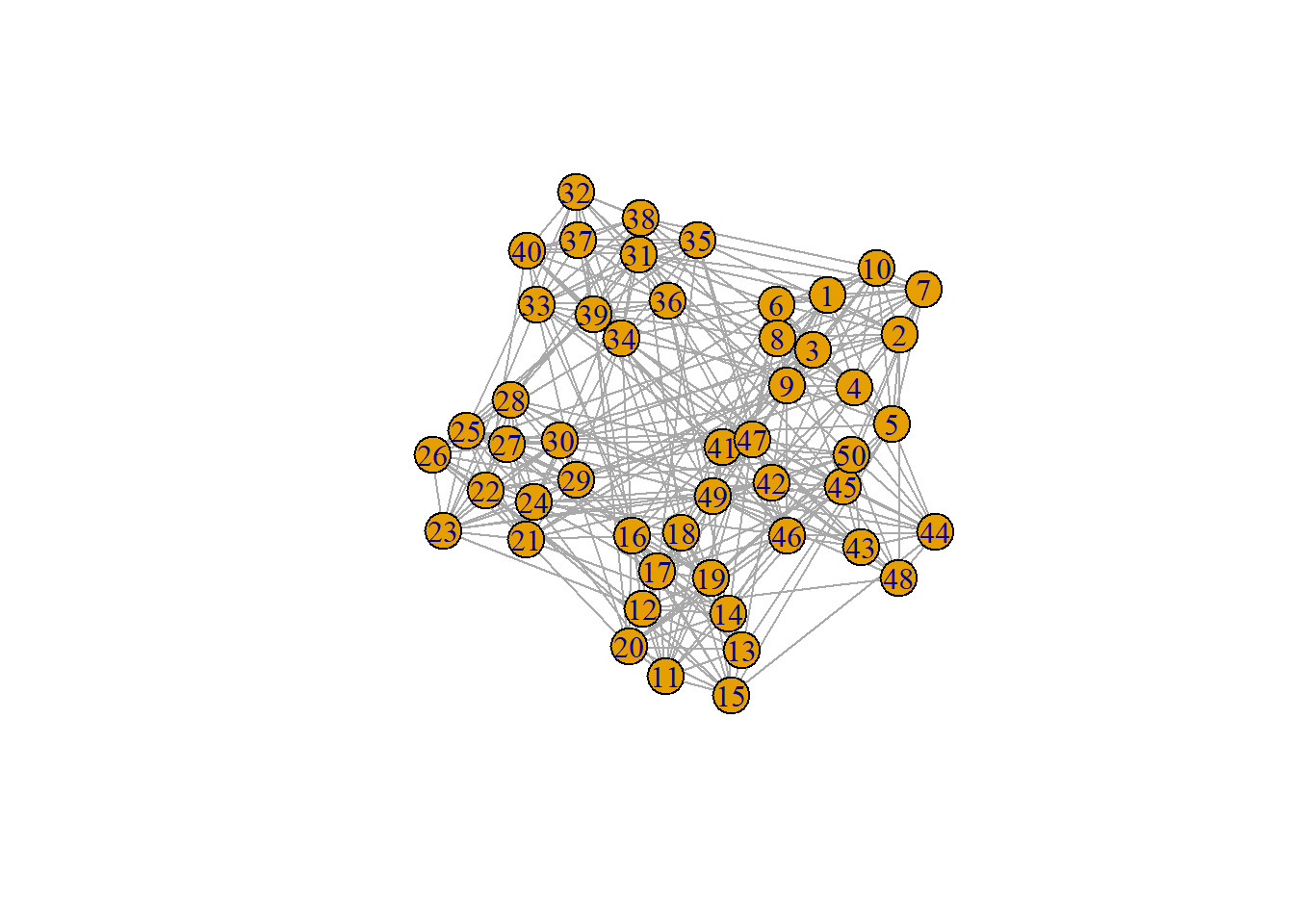
Step 1: Transition Matrix
The transition matrix, \(\mathbf{P}=\mathbf{D}^{-1}\mathbf{A}\), contains elements \(p_{ij}\) that represent the probability of a transition from vertex \(i\) to vertex \(j\) for a walk of length one (Brusco et al., 202413; Pons & Latapy, 200614). For a single vertex pair (\(i\) and \(j\)), the transition probability is \(P_{ij} = \frac{A_{ij}}{d(i)}\), where \(d(i) = \sum_{j} A_{ij}\). Walks of \(t\) length from vertex \(i\) to vertex \(j\) would be \(p_{ij}^t\).
The transition matrix is contingent on the number of “steps” expected to be taken, and the exponential form of \(\mathbf{P}^t\) represents this expanded transition matrix for \(t\) steps.
Thus, to arrive at the transition matrix, you will need both the adjacency matrix \(\mathbf{A}\) and the degree matrix \(\mathbf{D}\).
A Quick Note
Recall the “powers” of the adjacency matrix in Week 1, Adjacency Matrices. How does this relate to the notion of \(\mathbf{P}^t\)?
Step 2: Calculating Distance
Using both transition probabilities and degree, the distance (\(r(t)\)) between two vertices can be defined as the following:
\[r_{ij}(t) = \sqrt{\sum_{k=1}^p \frac{(p_{ik}^t - p_{jk}^t)^2}{d_{kk}}}\]
Distance can also be computed using elements of the data matrix \(\mathbf{X}^t\)15, and the formula can be extended to assessing the distance between two communities (\(r_{C_1C_2}\)). Computing distance is critical, as the objective function of the next step is to begin minimizing the sum of the squared (Euclidean) distances (SSE) between a member vertex and the centroid of a community.
Step 3: (Hierarchical) Clustering of the Distance Matrix
The actual ‘clustering’ portion of Walktrap is contingent upon an algorithm known as “Ward’s method” (Pons & Latapy, 2006)16. However, other clustering methods can be used (e.g., \(k\)-means clustering; Brusco et al., 2024b 17).
For now, we will focus on Ward’s method. The algorithm begins with treating each vertex as a single community. Then it assess whether or not to merge a community (\(C_1\)) with a second community (\(C_2\)). The choice on what communities to merge depends on whether the inevitable increase in SSE is minimized, or:
\[\Delta SSE(C_1, C_2) = \left(\frac{|C_1||C_2|}{|C_1| + |C_2|}\right)r^2_{C_1C_2}(t)\]
The iterative process hinges on two decision points: (1) when and how to merge two communities to optimize lower SSE, and (2) the final number of communities (\(K\)) to arrive at following a sequence of merges. With any given \(K\), there can be a large number of merge combinations that the computer has to consider when minimizing SSE, and the distance between communities must be re-computed after each marge. This makes the Ward method a computationally intensive process.
Once the hierarchical clustering algorithm arrives at \(K\) clusters, the quality of the partitions can be assessed.
groups = cluster_walktrap(ng) # default steps (t) is 4
plot(groups, ng)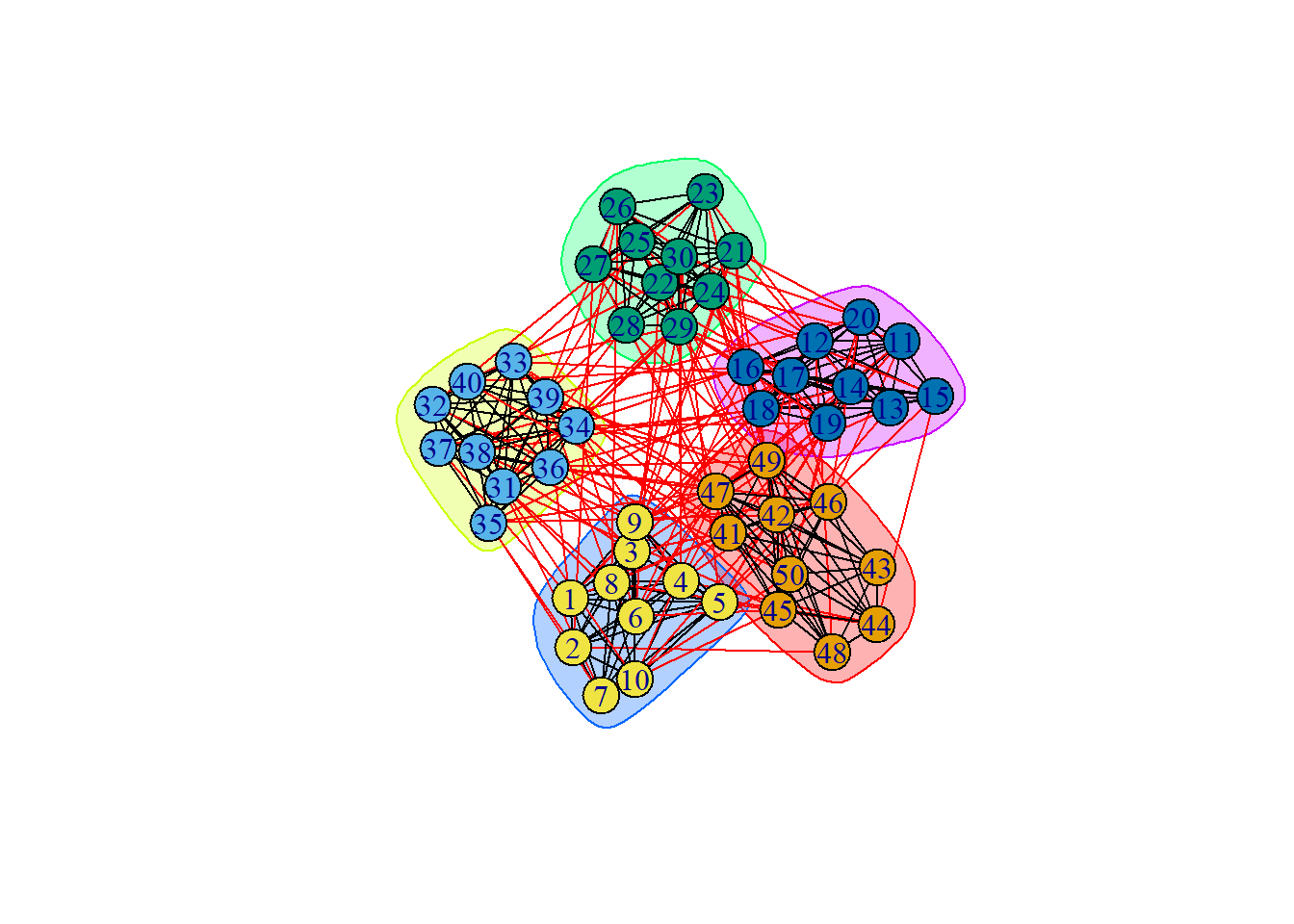
What happens when you change the number of steps (\(t\))?
groups2 = cluster_walktrap(ng, steps = 1)
plot(groups2, ng)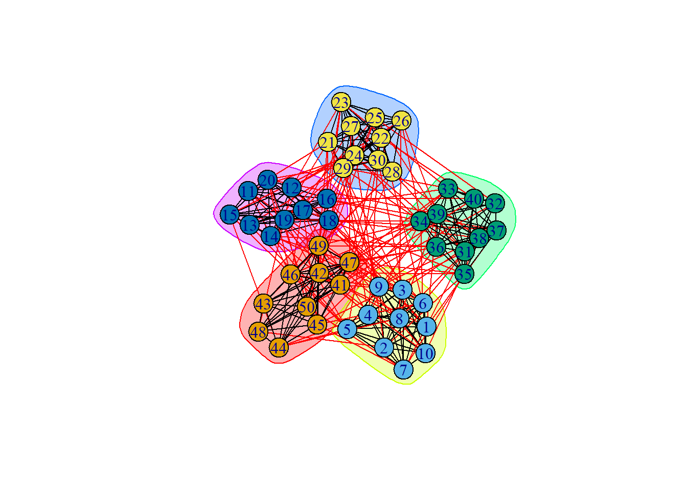
groups3 = cluster_walktrap(ng, steps = 30)
plot(groups3, ng)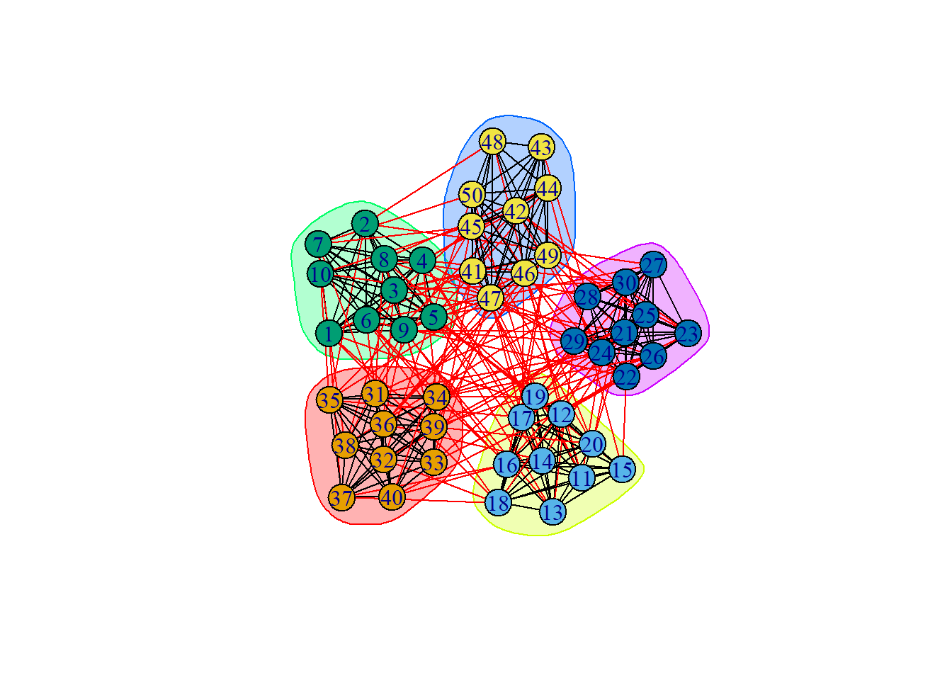
groups4 = cluster_walktrap(ng, steps = 1000)
plot(groups4, ng)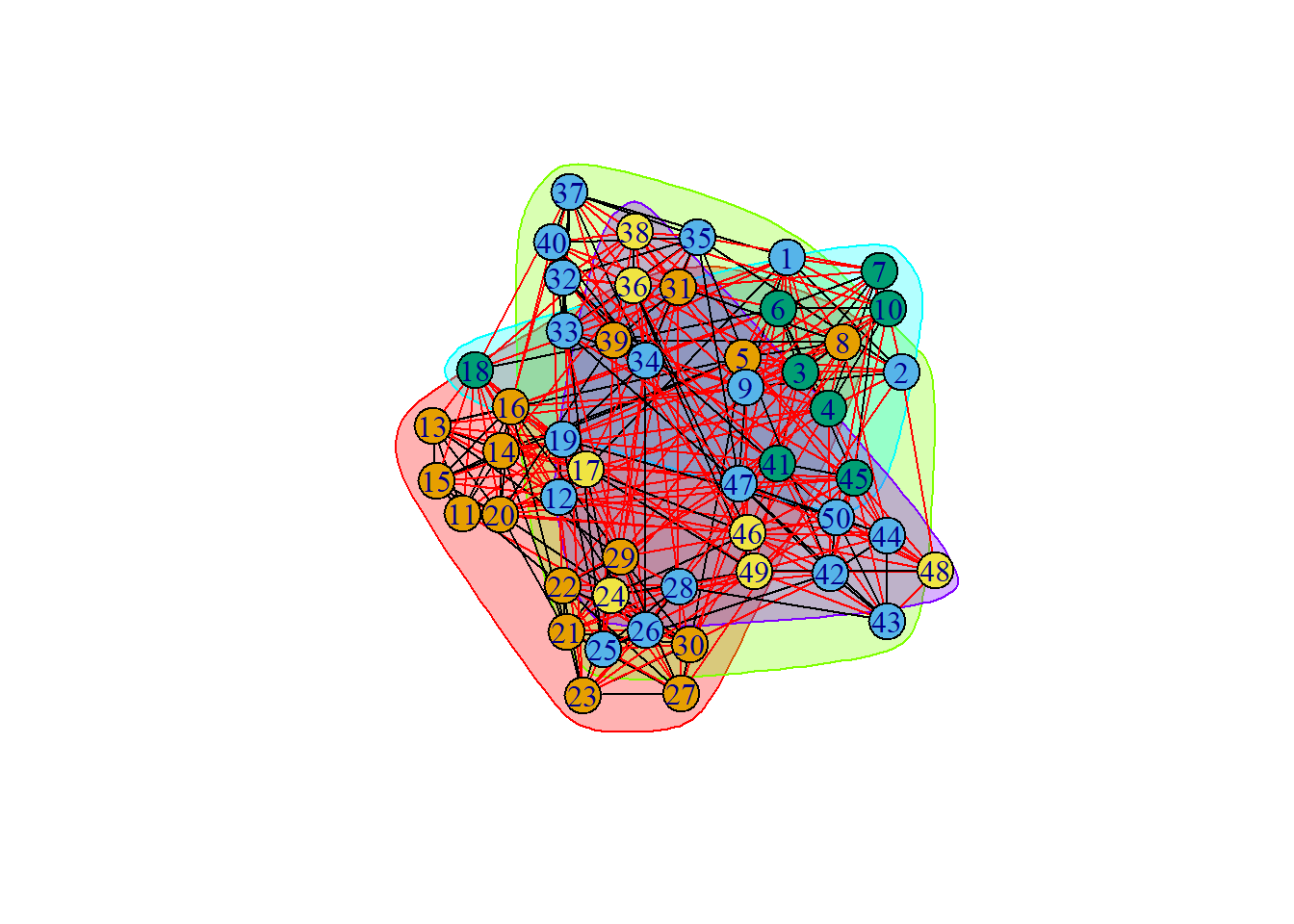
modularity(ng, # graph object
           membership(groups2) # extracting expected group membership of each node from results
)
[1] 0.4194097modularity(ng,
results.1[[5]][["cluster"]])[1] 0.4194097modularity(ng, membership(groups3)) [1] 0.4194097modularity(ng, membership(groups4))[1] 0.04381559# unsurprisingly, modularity is low for a high step count.Spectral Clustering
One of the final clustering methods that we will cover is spectral clustering. It is suitable for large networks, but the Walktrap algorithm has been shown to better identify community structures in network psychometrics (Brusco et al., 2024)18.
Spectral clustering both incorporates some potentially unfamiliar, such as eigenvalues and eigenvectors, and familiar concepts, such as k-means clustering. Let’s begin with the following:
\[\mathbf{A}v = \lambda v\]
- \(\mathbf{A}\) = adjacency matrix.
- \(v\) = the eigenvector that corresponds A to \(\lambda\), can represent a common dimension
- \(\lambda\) = the eigenvalue of \(\mathbf{A}\) (scalar), scales (lengthens or shortens) the values of \(v\)
The equivalency set up in the above equation poses the challenge of identifying the eigenvalues and eigenvectors that make that statement true. The number of maximal possible eigenvectors and values is limited by the number of total nodes in the network.
Conceptually, eigenvalues and eigenvectors are helpful information in identifying common dimensions of variance in a a dataset. Here is a site which demonstrates some basic principles of underlying dimensionality in 2D and 3D data: https://setosa.io/ev/principal-component-analysis/. While it discusses Principal Component Analysis (PCA), some of the principles remain the same.
Generally, larger eigenvalues indicate that shared variation in the data can be reduced to a common set of dimensions (i.e., principal components). However, we are interested in identifying local similarities within a network, as opposed to global similarities. This means we are interested in clustering eigenvectors in a way that captures shared variance within communities, rather than the network. The challenge arises in how we decompose our matrix of interest into meaningful groups via eigenvalues and eigenvectors.
This brings us to spectral clustering. There are a few ingredients we need to gather in order to perform spectral clustering. (Brusco et al., 2024b)19
First, we begin with something called a “Laplacian matrix”, which is the adjacency matrix subtracted from the degree matrix:
\[\mathbf{L} = \mathbf{D} - \mathbf{A}\]
- \(\mathbf{D}\) = diagonal matrix of degrees per node (\(d_i\); sum of edge weights)
- \(\mathbf{A}\) = adjacency matrix, with \(w_{ij}\) as edge weights
As noted in the code chunk for this section, we can derive a normalized Laplacian to appropriately scale the off-diagonal elements of the adjacency matrix{^brusco-2024b]. This has the unique property of normalizing vertices with small vertices. To do this, a \(p \times p\) identity matrix \(\mathbf{I}\), where \(p\) is the number of nodes.
\[\mathbf{L} = \mathbf{I} - \mathbf{D}^{-1}\mathbf{A}\]
A = adjacency.matrix
D.mat = diag(1/sqrt(degree(ng)), n.groups*n.nodes.per.group)
identity = diag(1, dim(D.mat))
Laplacian = identity - D.mat  %*% A %*% D.mat
Next, we extract eigenvectors of the Laplacian matrix, specifically the eigenvectors that correspond with the lower-tail end of eigenvalues.
k<-5 # specifying the number of groups
spectrum = eigen(Laplacian)$vectors[,((n.nodes.per.group*n.groups)-(k)):((n.nodes.per.group*n.groups)-1)]
Then, the eigenvectors must be clustered using some type of method. \(k\)-means clustering is an option. The number of clusters (\(k\)) must be specified.
spec.clust = kmeans(spectrum, centers = n.groups)

modularity(ng,
           spec.clust[["cluster"]])
[1] 0.3497106Summarizing Results
We’ve walked through an number of different approaches to identifying clusters, or “community detection”. The code demonstrations in each section used a simulated dataset. This means that we can compare the performance of each approach in recoverying the ‘true’ community structure. Since the community structure is known, we can use \(ARI_{HA}\) as our cluster quality index.
results = data.frame(Spectral = spec.clust$cluster,
                     k.Means = results.1[[n.groups]]$cluster,
                     c.Means = results.2[[n.groups]]$cluster,
                     # GMM = results.3$classification,
                     WalkTrap = groups$membership,
                     True = rep(1:n.groups, each = n.nodes.per.group))
ARIs = data.frame(Spectral = adjustedRandIndex(results$Spectral, results$True),
                  k.Means = adjustedRandIndex(results$k.Means, results$True),
                  c.Means = adjustedRandIndex(results$c.Means, results$True),
                  # GMM = adjustedRandIndex(results$GMM, results$True),
                  WalkTrap = adjustedRandIndex(results$WalkTrap, results$True))

ARIs
Spectral k.Means c.Means WalkTrap
1 0.804261 1 1 1Unsurprisingly, most of the approaches did great because they were ran with \(k\) equal to the true number of communities. The spectral clustering results lines up with past research, within it performing much worse than the Walktrap algorithm (Brusco et al., 2024b)20.
Issues With Psych Data
Network Size
- Gates et al., 2016: fMRI data as an example, smaller number of nodes, WalkTrap does great; used HA ARI and a Modularity Ratio because of DGP and Analytic Q
Clustering on Correlations
- Gates et al., 2016 MacMahon & Garlaschelli, 2014
- especially with time series data = linearly interdependent time series and temporal stationarity assumption
- null model, correlations get wonky, does other time series stuff related to industry-grouped stocks (does community composition change over time?)
- can focus on where correlations go wrong, and make a note of the other fun stuff in here (long paper)
Transparent Statement
we got help from GPT
Footnotes
Fortunato, S., & Barthélemy, M. (2007). Resolution limit in community detection. Proceedings of the National Academy of Sciences, 104(1), 36–41. https://doi.org/10.1073/pnas.0605965104↩︎
Pons, P., & Latapy, M. (2006). Computing Communities in Large Networks Using Random Walks. Journal of Graph Algorithms and Applications, 10(2), 191–218.↩︎
Steinley, D. (2006). K‐means clustering: A half‐century synthesis. British Journal of Mathematical and Statistical Psychology, 59(1), 1–34. https://doi.org/10.1348/000711005X48266↩︎
Gates, K. M., Henry, T., Steinley, D., & Fair, D. A. (2016). A Monte Carlo Evaluation of Weighted Community Detection Algorithms. Frontiers in Neuroinformatics, 10. https://doi.org/10.3389/fninf.2016.00045↩︎
Park, J.J., Chow, SM., Molenaar, P.C.M. (2024). What the Fuzz!? Leveraging Ambiguity in Dynamic Network Models. In: Stemmler, M., Wiedermann, W., Huang, F.L. (eds) Dependent Data in Social Sciences Research. Springer, Cham. https://doi.org/10.1007/978-3-031-56318-8_7↩︎
Fortunato, S., & Barthélemy, M. (2007). Resolution limit in community detection. Proceedings of the National Academy of Sciences, 104(1), 36–41. https://doi.org/10.1073/pnas.0605965104↩︎
Gates, K. M., Henry, T., Steinley, D., & Fair, D. A. (2016). A Monte Carlo Evaluation of Weighted Community Detection Algorithms. Frontiers in Neuroinformatics, 10. https://doi.org/10.3389/fninf.2016.00045↩︎
Fortunato, S., & Barthélemy, M. (2007). Resolution limit in community detection. Proceedings of the National Academy of Sciences, 104(1), 36–41. https://doi.org/10.1073/pnas.0605965104↩︎
MacMahon, M., & Garlaschelli, D. (2015). Community detection for correlation matrices. Physical Review X, 5(2), 021006. https://doi.org/10.1103/PhysRevX.5.021006↩︎
MacMahon, M., & Garlaschelli, D. (2015). Community detection for correlation matrices. Physical Review X, 5(2), 021006. https://doi.org/10.1103/PhysRevX.5.021006↩︎
Park, J.J., Chow, SM., Molenaar, P.C.M. (2024). What the Fuzz!? Leveraging Ambiguity in Dynamic Network Models. In: Stemmler, M., Wiedermann, W., Huang, F.L. (eds) Dependent Data in Social Sciences Research. Springer, Cham. https://doi.org/10.1007/978-3-031-56318-8_7↩︎
park-2024↩︎
Brusco, M., Steinley, D., & Watts, A. L. (2024). Improving the Walktrap Algorithm Using K-Means Clustering. Multivariate Behavioral Research, 59(2), 266–288. https://doi.org/10.1080/00273171.2023.2254767↩︎
Pons, P., & Latapy, M. (2006). Computing Communities in Large Networks Using Random Walks. Journal of Graph Algorithms and Applications, 10(2), 191–218.↩︎
Brusco, M., Steinley, D., & Watts, A. L. (2024). A comparison of spectral clustering and the walktrap algorithm for community detection in network psychometrics. Psychological Methods, 29(4), 704–722. https://doi.org/10.1037/met0000509↩︎
Brusco, M., Steinley, D., & Watts, A. L. (2024). A comparison of spectral clustering and the walktrap algorithm for community detection in network psychometrics. Psychological Methods, 29(4), 704–722. https://doi.org/10.1037/met0000509↩︎
Brusco, M., Steinley, D., & Watts, A. L. (2024). A comparison of spectral clustering and the walktrap algorithm for community detection in network psychometrics. Psychological Methods, 29(4), 704–722. https://doi.org/10.1037/met0000509↩︎
Brusco, M., Steinley, D., & Watts, A. L. (2024). A comparison of spectral clustering and the walktrap algorithm for community detection in network psychometrics. Psychological Methods, 29(4), 704–722. https://doi.org/10.1037/met0000509↩︎