Understanding the type of data we are working with is crucial before selecting or designing in psychological and behavioral sciences. Different data types influence which modeling frameworks are most appropriate.
Broadly, psychological research data can be categorized into:
Continuous:
Interval (e.g., temperature, standardized scores)
Ratio (e.g., reaction time, height)
Discrete:
Categorical
Nominal (e.g., gender, treatment conditions)
Ordinal (e.g., Likert scale responses, grade)
Count (e.g., number of behavioral occurrences)
Binary (yes/no, present/absent, true, false)
Regular Graphs
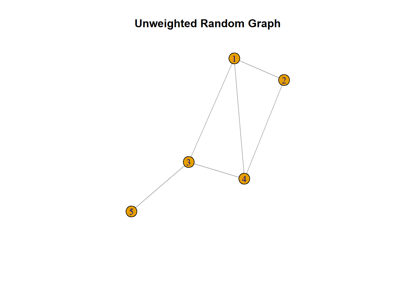
Regular graphs typically utilize binary data, represented by edges that indicate either the presence (1) or absence (0) of a relationship. This binary representation simplifies modeling and interpretation of direct relationships between nodes. Common examples include adjacency matrices, where a cell entry of “1” denotes a connection (two nodes are linked) and “0” denotes no connection. Such binary networks are particularly useful in psychological research for modeling symptom networks, behavioral co-occurrences, or communication patterns.
Below is an example regular graph
library(igraph)set.seed(4399)g1 <-sample_gnp(n =5, p =0.5)adj_matrix <-as_adjacency_matrix(g1, sparse =FALSE)plot(g1, main ="Unweighted Random Graph")
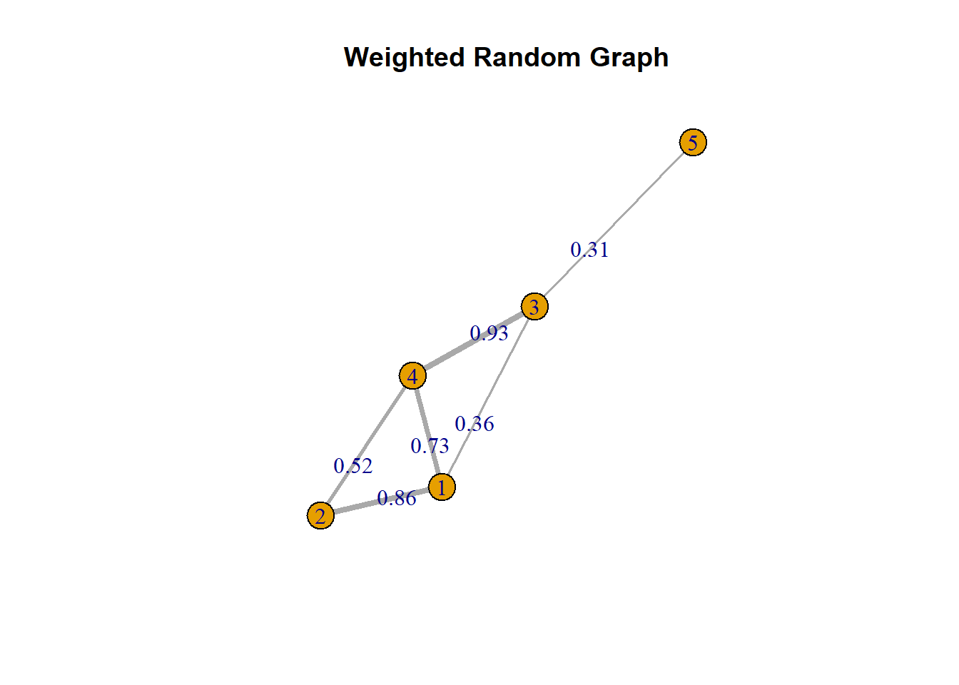
Many psychological phenomena are more realistically represented by continuous relationships, which vary in intensity or strength. Weighted networks extend binary graphs by assigning numeric weights to edges, reflecting the magnitude of interaction or connection strength between nodes.
These weights may reflect:
Correlation or partial correlation coeffcients
Time-lagged associations in temporal data
In psychological research, weighted networks are used in a variety of contexts, including:
Partial correlation networks: Edges depict conditional dependencies among variables, controlling for all others.
Dynamic/Temporal networks: Edges represent lagged or dynamic relationships between psychological variables, helping model how states evolve over time.
Compared to binary networks, weighted networks preserve more information, enabling richer analyses (e.g., edge centrality, strength-based clustering).
Here’s an example of a weighted graph
# Assign random weights (e.g., between 0.1 and 1) to each edgeE(g1)$weight <-runif(ecount(g1), min =0.1, max =1.0)E(g1)$label <-round(E(g1)$weight, 2)E(g1)$width <-E(g1)$weight *5plot(g1, edge.label =E(g1)$label, main ="Weighted Random Graph")
While weighted networks capture nuanced variation and continuous relationships, foundational models often begin with binary graphs, where relationships are represented as present or absent, and node states are either “on” or “off.” These binary forms are not just simplifications, but reflect an essential class of systems in psychology and biology that operate in discrete states (e.g., yes/no, active/inactive).
We’ve discussed how weighted networks extend binary ones by encoding strength or intensity. However, not all phenomena benefit from continuous modeling. Finer and finer gradients of analysis, though numerically tractable, may fail to reflect the categorical nature of many real-world transitions.
For example:
Is someone depressed or not? (vs. how depressed are they?)
Does a student have a satisfactory academic standing? (vs. whether they have an A- or a B+)
Has a person acted on a decision? (vs. how close they were to doing so)
In such cases, binary models may offer cleaner interpretability and emphasize psychologically meaningful thresholds rather than arbitrary numerical scales. Boolean systems, in particular, allow us to capture how such states evolve through clear logical rules.
Limitations of Current Binary Models
Despite their interpretability, binary models also come with limitations, especially in psychological research:
Many binary models, such as the Ising model, are designed for cross-sectional data. They can describe static relationships (e.g., symptom presence) but fail to capture temporal dynamics: how systems change and evolve over time.
There is no widely adopted framework for modeling the time-dependent structure of binary psychological networks.
This limits our ability to study how binary states (e.g., on/off, active/inactive) unfold across time, particularly in systems governed by rule-based or threshold dynamics.
Boolean networks address this gap. They offer a formal structure to model the temporal evolution of binary systems using logic-based update functions. This makes them particularly suitable for modeling:
Gene regulation
Belief revision
Habitual behavior and behavioral switching
Boolean networks thus extend the utility of binary models beyond static relationships, into the realm of dynamic system modeling.
Boolean Networks
Brief History
Boolean networks were originally introduced by Stuart Kauffman in 1969 as a model for understanding how complex biological order can emerge from random systems. Rather than relying on detailed, continuous equations or coded descriptions, Kauffman proposed that simple binary rules, where variables take on either an “on” (1) or “off” (0) state, could explain how patterns of activity evolve over time.
Kauffman’s key insight was that continuous biological systems (like gene expression) could be approximated by discrete binary systems, where each gene is either active or inactive, and its behavior depends on a set of logical rules defined by other genes. This abstraction made it possible to simulate large networks and explore emergent behaviors such as homeostasis, differentiation, and self-organization.
One of the most important concepts in Kauffman’s model is the idea of a stable (equilibrium) state, where the system settles into a pattern, often representing distinct cell types. Even when parts of the system (e.g., individual nodes or genes) are perturbed, the network often returns to its original cycle or fixed point, suggesting inherent robustness in biological systems.
Low network connectivity was shown to favor stability, while higher connectivity could lead to chaotic or unstable behavior, drawing an early link between network structure and dynamics.
Adoption into Other Fields
Boolean networks were initially used to model gene regulatory networks in biology, but their influence has since extended to many other fields. Because many complex systems can be simplified into binary components and rule-based interactions, Boolean networks offer a natural modeling approach for:
Neural activation and inhibition
Decision-making and belief systems
Social influences and behavior switching
Computational modeling of disease spread, political dynamics, and emotion regulation
In essence, Boolean networks provide a simple but powerful formalism for studying how binary variables interact over time to create complex, emergent behaviors in dynamical systems.
Binary Data as the Foundation of Boolean Networks
A binary variable is one that has exactly two possible states, typically represented as 0 or 1, OFF or ON, False or True, or any other two-level distinction. By combining multiple binary variables and defining how they influence each other, we can simulate complex dynamic systems.
How Binary Works: Counting in Binary
Binary numbers follow a base-2 system, where each digit (called a bit) represents an increasing power of 2, from right to left. Here’s how we count from 0 to 7 using 3 binary digits (bits):
000 = 0
001 = 1
010 = 2
011 = 3
100 = 4
101 = 5
110 = 6
111 = 7
Each bit can only be 0 or 1, but combining bits exponentially increases the number of possible states. For example:
1 bit → 2 states (0, 1)
2 bits → 4 states (00, 01, 10, 11)
3 bits → 8 states
\(n\) bits → \(2^n\) possible states
This idea is central to Boolean networks: a system of \(n\) binary nodes can exist in one of \(2^n\) possible configurations/states at any given time.
Question:
What is the digit configuration of 9 in binary format?
Boolean Logic Rules
Boolean networks operate on simple logical operations, called Boolean rules, that govern how each node updates its state (0 or 1) based on the states of its input nodes. These rules are rooted in classic logic gates, commonly used in digital circuits and computation.
The three most fundamental Boolean rules are:
AND ( ∧ ): Returns 1 (True) only if all inputs are 1.
| A | B | A ∧ B |
|---|---|-------|
| 0 | 0 |   0   |
| 0 | 1 |   0   |
| 1 | 0 |   0   |
| 1 | 1 |   1   |
OR ( ∨ ): Returns 1 if at least one input is 1.
| A | B | A ∨ B |
|---|---|--------|
| 0 | 0 |   0    |
| 0 | 1 |   1    |
| 1 | 0 |   1    |
| 1 | 1 |   1    |
NOT ( ¬ ): Takes a single input and inverts it.
| A | ¬A |
|---|----|
| 0 | 1  |
| 1 | 0  |
Boolean Rules Can Be Combined:
In real Boolean networks, nodes often use combinations of multiple logic operations to define their update rules, creating more flexible and plausible dynamics.
Here are some sample rule that involves AND, OR, and NOT: D = (A ∧ B) ∨ (¬C) D = ¬(A ∨ B) D = (A ^ ¬B) ∨ (¬A ^ B) Note: Sometimes (A ^ ¬B) ∨ (¬A ^ B) is simplified as A ⊕ B. ⊕ or XOR (exclusive OR) returns 1 if and only if one input is 1.
These rules form the core update logic in Boolean networks. Each node applies one of these rules (or a combination of them) to determine its next state based on the current states of its input nodes.
The Boolean Network Model
As we discussed earlier, a Boolean network is a system composed of binary variables (nodes), each of which updates its value over time based on a specified Boolean function of other nodes in the system. These logical rules define the edges (connections) in the network, determining which nodes influence which.
Boolean networks may appear simple, but they can give rise to rich dynamics over time. Even small networks can settle into stable states where node values no longer change, a property often interpreted as modeling homeostasis or equilibrium in the system.
Discrete Time and Synchronous Updates
Time progresses in discrete steps. At each time step \(t\), all nodes update their state simultaneously based on their input nodes. (We will assume synchronous updating for now, and will discuss different updating scheme later)
Boolean Network as a Graph
A Boolean network can be visualized as a directed graph, where:
Edges represent dependencies — i.e., which nodes influence which
Each node is associated with a Boolean function that defines its next value
Formulation
Let’s define a Boolean network formally: \[ G(X(t), B) \]
Let \[ X(t) = \{x_1(t), x_2(t), \dots, x_n(t)\} \]
be the state of all \(n\) nodes at time \(t\).
Let \[ B = \{f_1, f_2, \dots, f_n\} \]
be the set of Boolean functions assigned to each node.
Each node updates according to: \[ X_i(t+1) = f_i(X_{i1}(t), X_{i2}(t), \dots, X_{ik}(t)) \]
where \(X_{i1}, \dots, X_{ik}\) are the input nodes for \(X_i\).
Example Boolean Update Rules
Suppose we have a 3-node Boolean network with the following rules:
Attractor 1 is a simple attractor consisting of 1 state(s) and has a basin of 1 state(s):

 |--<--|
 V     |
 000   |
 V     |
 |-->--|


Genes are encoded in the following order: X1 X2 X3

Attractor 2 is a simple attractor consisting of 1 state(s) and has a basin of 4 state(s):

 |--<--|
 V     |
 001   |
 V     |
 |-->--|


Genes are encoded in the following order: X1 X2 X3

Attractor 3 is a simple attractor consisting of 2 state(s) and has a basin of 3 state(s):

 |--<--|
 V     |
 010   |
 101   |
 V     |
 |-->--|


Genes are encoded in the following order: X1 X2 X3
This small example already demonstrates how logical dependencies can create feedback loops and stable configurations.
What are Attractors?
In Boolean networks, attractors represent the long-term behavior of the system. No matter where the system starts, it will eventually settle into one of these stable patterns, either:
A fixed point (a single unchanging state), or
A limit cycle (a repeating sequence of states)
Because Boolean networks are:
Deterministic (no randomness in updates), and
Have a finite number of global states (for \(N\) binary nodes, there are \(2^N\) possible states),
The system is guaranteed to eventually repeat a state or a set of states. This repetition defines an attractor.
Intuition: Attractors as Stable Patterns You can think of attractors as:
Habitual behaviors in psychology,
Stable configurations in gene regulation, or
Homeostatic states in dynamic systems.
Regardless of where the system starts, its internal logic will guide it toward one of these stable states or cycles over time.
State Space and State Transition Graphs
For a Boolean network with \(N\) nodes, there are \(2^N\) possible global states.
For example, if \(N = 3\), the global states are: 000, 001, 010, 011, 100, 101, 110, 111
A state transition graph maps how the system evolves:
Each node in the graph represents a global state (e.g., 101).
Each arrow (edge) represents how the state changes after applying the Boolean update rules.
Because the system is deterministic, every state has exactly one outgoing arrow — leading to a unique next state.
How Attractors Emerge From any starting point, the system follows a deterministic trajectory through the state space. Eventually, it must:
Loop back to a previously visited state, or
Settle into a state that maps onto itself
These are the attractors.
Types of Attractor
Fixed Point (Point Attractor)
A single stable state that maps onto itself: 101 → 101 → 101…
Limit Cycle (Cyclic Attractor)
A repeating sequence of states: 010 → 110 → 010…
Complex Attractor
A longer or less regular sequence (rare in simple Boolean models)
Basins of Attraction
Each attractor has a basin of attraction — the set of starting states that eventually flow into it.
For example:
If states 000, 001, and 010 all end up in attractor 111, they all belong to the basin of 111.
Basins help us understand how different initial conditions converge to the same long-term outcome.
Why Are Attractors Important?
Attractors offer insight into the predictable outcomes of complex systems. They help us:
Analyze long-term behavior
Understand system stability
Explore how different conditions converge or diverge
In psychological and biological systems, attractors can be interpreted as:
Habitual thought or behavior patterns
Emotional regulation states
Gene expression profiles
Construction of Boolean Networks
Once we understand the basic structure of a Boolean network — nodes, logical rules, and state transitions — the next step is to ask: How do we actually build one from data?
There are two general approaches:
Theory-driven construction:
You specify the Boolean rules based on prior knowledge of the system (e.g., known gene interactions or logical hypotheses in psychology).
Data-driven inference:
You infer the logical rules from observational or experimental data using algorithms that search for the best-fitting Boolean functions.
Guiding Principles for Construction
Parsimony: Choose the simplest possible model that fits the data well. Simpler networks are easier to interpret and less prone to overfitting.
Best-fitting: Among candidate rule sets, select those that explain the observed transitions or outcomes most accurately (those that lead to fewest false positives and false negatives)
Limited Input Size:
When inferring rules from data, we often limit the number of inputs per node (i.e., how many other nodes influence a given node). This helps reduce model complexity and improve interpretability.
A common default is: \(\text{maxK} = 2\). Meaning no node is influenced by more than two others — a reasonable assumption when theory is limited or noisy.
Number of Boolean Functions with \(k\): why limiting \(maxK\)
The number of distinct Boolean functions a node can have depends on the number of its input variables \(k\). For each combination of inputs, a Boolean function assigns either 0 or 1 as output. Since there are \(2^k\) possible input combinations and each combination can map to 0 or 1, the total number of possible Boolean functions is \(2^{2^k}\)
Examples:
With 1 input: \(2^{2^1}\) = 4 functions
With 2 inputs: \(2^{2^2}\) = 16 functions
With 3 inputs: \(2^{2^3}\) = 256 functions
This exponential growth reflects the expressive power of Boolean functions, even with few inputs.
Inference Examples (Small k)
When \(k = 1\):
Rules like \(x_1(t+1) = ¬X3(t)\) or \(x_3(t+1) = x_3(t)\) (simple dependence)
When \(k = 2\): Allows more expressive logic such as \(x_1(t+1) = x_2(t) ∧ x_3(t)\) or \(x_2(t+1) = ¬x_2(t) ∨ x_1(t)\)
These restrictions help identify the most likely mechanisms behind observed data patterns, without introducing too many assumptions.
Update Scheme
In a Boolean network, the update scheme determines how the system evolves over time, specifically, how and when nodes update their states.
Synchronous Updating
In synchronous updating, all nodes compute their new values simultaneously at each time step. The update from time \(t\) to \(t+1\) is based on the state of the network at time \(t\).
This is the default assumption in most introductory Boolean models. It’s simple, deterministic, and easy to analyze.
Asynchronous Updating
In asynchronous updating, nodes update one at a time, or in subsets, rather than all at once. This can better reflect real-world systems where changes don’t happen simultaneously.
Common Variants:
Deterministic asynchronous: Nodes update in a fixed, repeating order.
Stochastic asynchronous: A node is chosen at random at each time step.
Random-order asynchronous: All nodes are updated once per time step, but in a random sequence.
General asynchronous: Each node has a specific probability of being selected, which may be unequal.
Why It Matters: Key Differences
In synchronous models, each state has exactly one successor.
In asynchronous models, one state can lead to multiple possible next states, depending on the update order.
This can lead to important changes in the network’s dynamics:
Attractors can change: Some cyclic attractors (limit cycles) may disappear or transform.
Basins may split: A single initial state may lead to multiple possible attractors under different update paths.
Limit cycles may vanish in favor of convergence to fixed points or more complex behavior.
Fixed-point attractors are often preserved.
Open Questions for Reflection
What does asynchronous updating better model in the real world?
How might randomness or timing affect system stability?
Are fixed points always robust under update scheme changes?
Network Control
Once a Boolean network is constructed, a natural question arises: Can we steer the system toward a desired behavior or away from an undesirable one?
This is the goal of network control: applying perturbations or interventions to change the long-term dynamics of the system.
Types of Interventions
Several strategies exist for controlling Boolean networks, each altering the network in different ways:
Node deletion: Remove a node entirely from the network — useful for modeling knockout experiments or loss of function.
Node override: Force a node to stay in a fixed state (e.g., always ON or always OFF), overriding its logical rule. Common in therapeutic modeling.
Edgetic control: Modify or remove specific edges (influences) between nodes, rather than the nodes themselves, e.g., block a specific regulatory interaction. The effect is usually more targeted and local.
These interventions can redirect the system from one attractor to another, ideally from an undesirable state (e.g., disease) to a stable, healthy one.
Hamming Distance and Control Planning
To evaluate how hard it is to shift from one state to another, we use Hamming distance:
The Hamming distance between two binary states is the number of bits (nodes) that differ between them.
In network control, it’s often used to measure:
The distance between an undesired attractor and the basin of a more desirable attractor
The minimum number of node changes needed to redirect the system
This helps in designing minimal interventions that are most efficient and least disruptive.
Conceptual Applications
In biology: Can we suppress a disease pathway by targeting just one gene or edge?
In psychology: Can we identify key factors that break a cycle of maladaptive behavior?
In policy/sociology: Can a small intervention in one part of a social network tip the system toward a more desirable equilibrium?
How to do this in \(\texttt{R}\)
Packages needed for Boolean network
library(BoolNet)library(igraph)
Generating a Random Boolean Network
# Generating a random "N-K"# N = Number of Nodes# K = Average Degree of each Nodeset.seed(256)N =3net =generateRandomNKNetwork(n = N, k =2, topology ="homogeneous", linkage ="uniform", functionGeneration ="uniform",noIrrelevantGenes =FALSE, simplify =TRUE,readableFunctions =TRUE)# Set readableFunctions = TRUE to display transition functions # in human-readable Boolean format (e.g., A & B), instead of binary vectors.# We will also learn how to interpret the transition functions in binary format later# Rename Variablesnet$genes =c("Slacking Off", "Happy Advisor", "Rewarded")# How are Boolean Rules Defined here?net
Boolean network with 3 genes

Involved genes:
Slacking Off Happy Advisor Rewarded

Transition functions:
Slacking Off = (!Gene3 & !Gene1)
Happy Advisor = (!Gene1)
Rewarded = (Gene2)
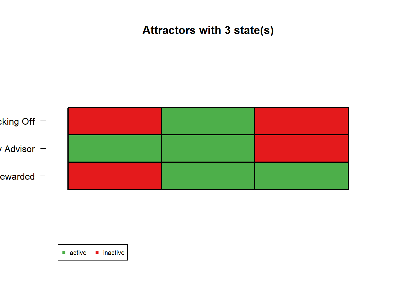
Attractors =getAttractors(net)Attractors
Attractor 1 is a simple attractor consisting of 1 state(s) and has a basin of 1 state(s):

 |--<--|
 V     |
 011   |
 V     |
 |-->--|


Genes are encoded in the following order: Slacking Off Happy Advisor Rewarded

Attractor 2 is a simple attractor consisting of 3 state(s) and has a basin of 7 state(s):

 |--<--|
 V     |
 010   |
 111   |
 001   |
 V     |
 |-->--|


Genes are encoded in the following order: Slacking Off Happy Advisor Rewarded
# Method provides the results that best describe the data even if there are some errorsrecon =reconstructNetwork(bin, method ="bestfit",maxK = N-1,returnPBN =FALSE,readableFunctions =FALSE)recon
Probabilistic Boolean network with 3 genes

Involved genes:
Slacking Off Happy Advisor Rewarded

Transition functions:

Alternative transition functions for gene Slacking Off:
Slacking Off = <f(Slacking Off,Rewarded){0010}> (error: 220)

Alternative transition functions for gene Happy Advisor:
Happy Advisor = <f(Slacking Off,Rewarded){1101}> (error: 229)

Alternative transition functions for gene Rewarded:
Rewarded = <f(Happy Advisor,Rewarded){0111}> (error: 231)
Disregard the error rate for now. Above, you see the transition functions in the binary format:
    Slacking off = f(Slacking Off, Rewarded){0010}
      The progression of the binary digits is:
        Slacking off = 0 and Rewarded = 0 = 0
        Slacking off = 0 and Rewarded = 1 = 0
        Slacking off = 1 and Rewarded = 0 = 1
        Slacking off = 1 and Rewarded = 1 = 0
    Happy Advisor = <f(Slacking Off,Rewarded){1101}
      The progression of the binary digits is:
        Slacking off = 0 and Rewarded = 0 = 1
        Slacking off = 0 and Rewarded = 1 = 1
        Slacking off = 1 and Rewarded = 0 = 0
        Slacking off = 1 and Rewarded = 1 = 1
    Rewarded = <f(Happy Advisor,Rewarded){0111}
      The progression of the binary digits is:
        Happy Advisor = 0 and Rewarded = 0 = 0
        Happy Advisor = 0 and Rewarded = 1 = 1
        Happy Advisor = 1 and Rewarded = 0 = 1
        Happy Advisor = 1 and Rewarded = 1 = 1
Probabilistic Boolean network with 3 genes

Involved genes:
Slacking Off Happy Advisor Rewarded

Transition functions:

Alternative transition functions for gene Slacking Off:
Slacking Off = (Slacking Off & !Rewarded) (error: 220)

Alternative transition functions for gene Happy Advisor:
Happy Advisor = (!Slacking Off) | (Rewarded) (error: 229)

Alternative transition functions for gene Rewarded:
Rewarded = (Rewarded) | (Happy Advisor) (error: 231)
Let’s switch back to the human readable version. You can see that recon now has intuitive functions to interpret again:
    Slacking Off = (Slacking Off & !Rewarded)
    When we slacked off AND didn't feel rewarded at the previous time, we continue to slack off

    Happy Advisor = (!Slacking Off) | (Rewarded)
    When we didn't slack off OR felt rewarded at the previous time, our advisor becomes happy.

    Rewarded = (Rewarded) | (Happy Advisor)
    We will feel rewarded again if we felt rewarded OR our advisor was happy at the previous time.
Questions:
How is our fitted model compared to our original model?
What do you think of the error rate?
Sometimes, we get multiple alternative transition functions, and we only would like to keep one. The current example doesn’t have multiple transition functions. But keep in mind that it could happen.
Boolean network with 3 genes

Involved genes:
Slacking Off Happy Advisor Rewarded

Transition functions:
Slacking Off = (Slacking Off & !Rewarded)
Happy Advisor = (!Slacking Off) | (Rewarded)
Rewarded = (Rewarded) | (Happy Advisor)
Obtaining Attractors
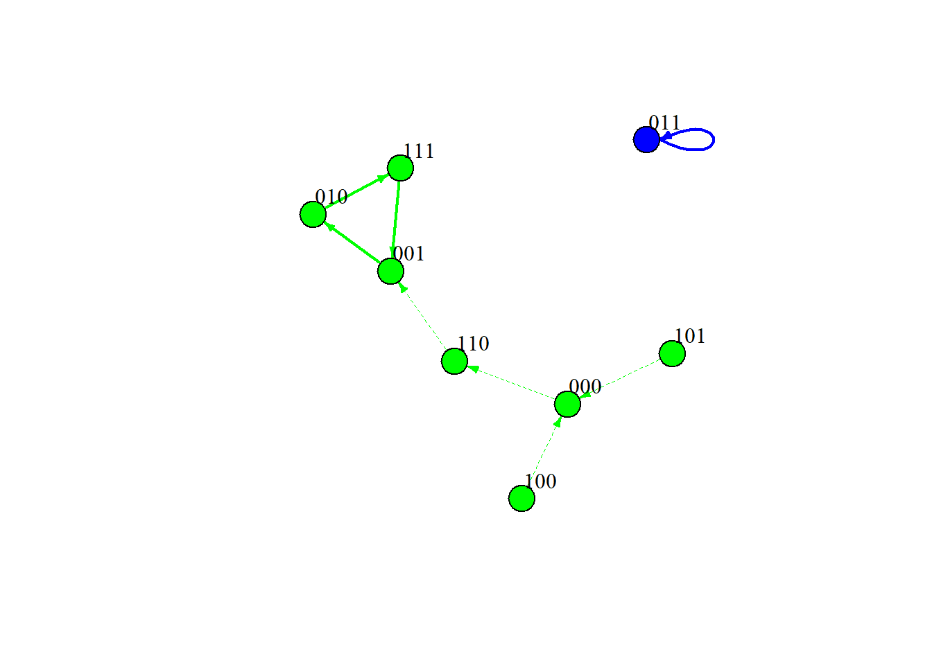
ga =getAttractors(network = singlenet, type ="synchronous",returnTable =TRUE)ga
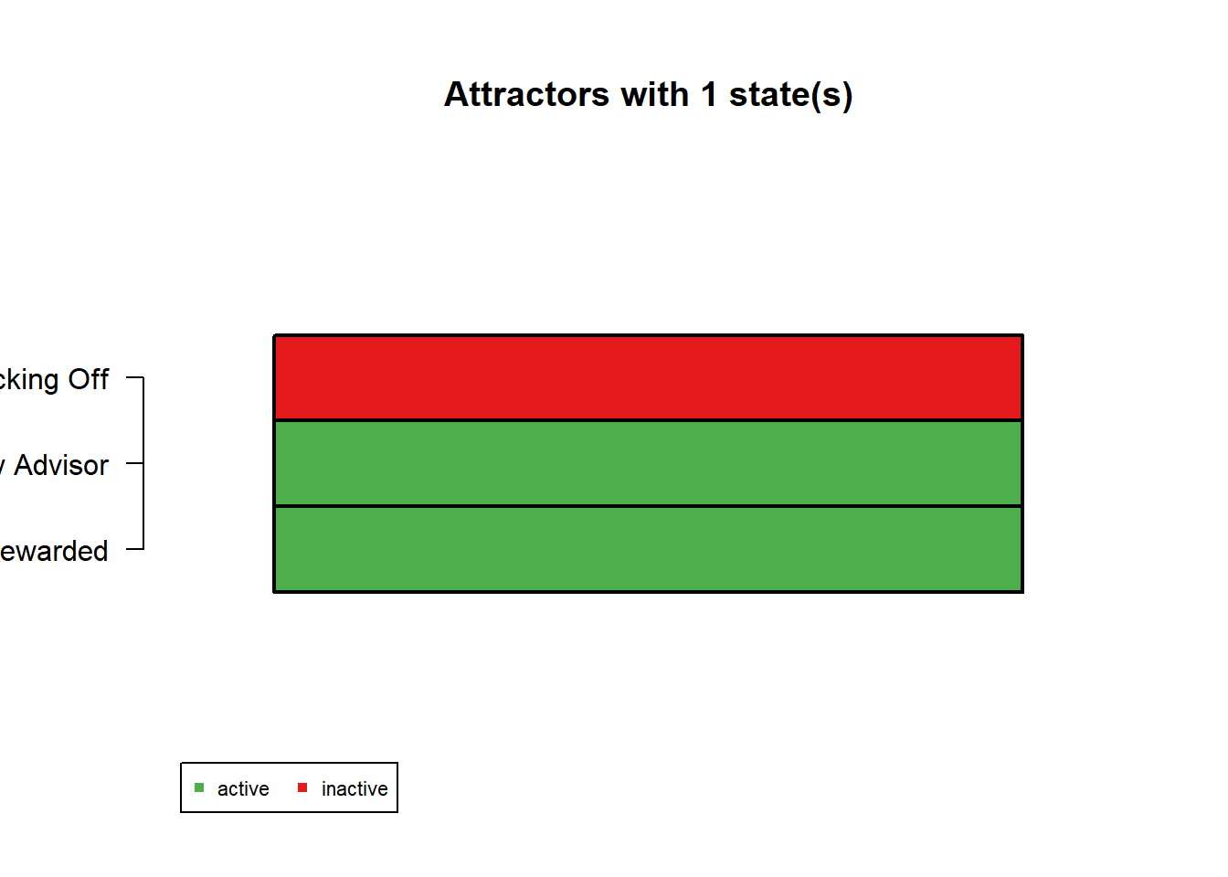
Attractor 1 is a simple attractor consisting of 1 state(s) and has a basin of 7 state(s):

 |--<--|
 V     |
 011   |
 V     |
 |-->--|


Genes are encoded in the following order: Slacking Off Happy Advisor Rewarded

Attractor 2 is a simple attractor consisting of 1 state(s) and has a basin of 1 state(s):

 |--<--|
 V     |
 100   |
 V     |
 |-->--|


Genes are encoded in the following order: Slacking Off Happy Advisor Rewarded
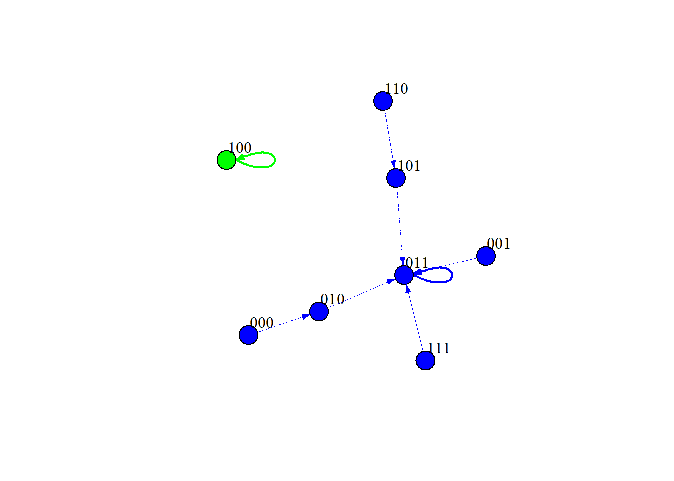
# Asynchronous update randomly selects a node and updates it contingent on the state of the system at the moment it is updated# Can also find complex or "loose" attractors that govern a systemga2 =getAttractors(network = singlenet, type ="asynchronous")ga2
Attractor 1 is a simple attractor consisting of 1 state(s):

 |--<--|
 V     |
 011   |
 V     |
 |-->--|


Genes are encoded in the following order: Slacking Off Happy Advisor Rewarded
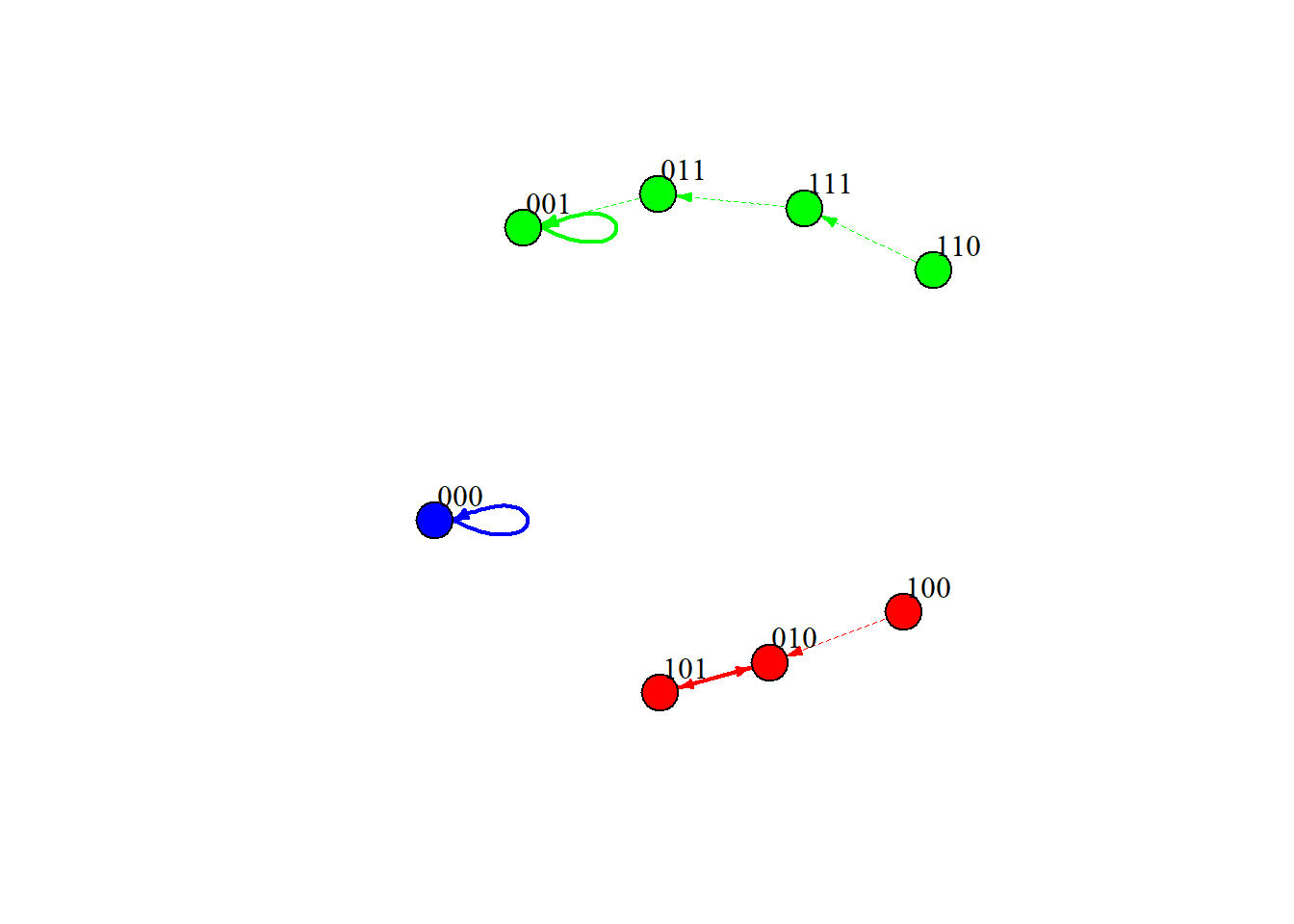
Let’s see how the state transition graph from our reconstructed model looks like
For the synchronous update, we can see that the steady state attractor is:
    011: When we never slack off, and our advisor is always happy
         and we always feel rewarded
    100: When we slack off all the time,
         and our advisor never feels happy and we never feel rewarded
Question: How would you interpret the model?
Reflection/Discussion Questions
How do people think of binarization of continuous data?
When is Boolean Network appropriate to use? What is its benefits & costs?
Can all psychological phenomona be modeled as discrete?
Any comments or questions on the readings or Boolean network in general?