Centrality Metrics

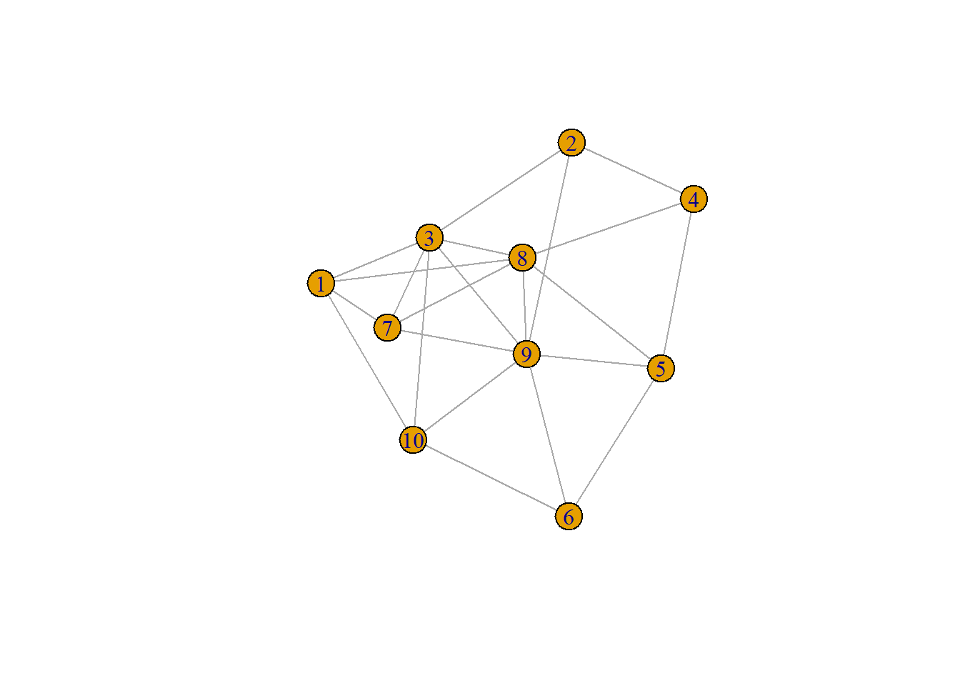
Welcome to the second week of our Network Analysis seminar.

Recap

Last week, we covered the basics of defining a graph based on the vertex set, \(V\), and the edgelist, \(E\). We also learned that the maximum cardinality of our edgelist, \(|E|_{max}\) is constrained both by its own definition but also by \(|V|\). For an undirected simple graph, \(|E|_{max}\) was given by:

\[|E|_{max} = \frac{|V|(|V|- 1)}{2}\]

By contrast, in a digraph, \(|E|_{max}\) was given by:

\[|E|_{max} = |V|^2\]

We never formally expressed the cardinality of a multigraph for reasons that should be self-evident. If they are not, let’s revisit that. Recall, our definition of an undirected multigraph was given by:

\[G = (V, E)\]

where \(V\) is a set of vertices and \(E\) is given by:

\[E \subseteq \{(\{x,y\},i) |x, y \in V, i \in \mathbb{N}\}\]

In this case, \(i\) can take the form of any of the natural numbers, \(\mathbb{N}\). This means that the maximum cardinality of \(E\) is constrained not by the cardinality of the vertex list but rather by the cardinality of the natural numbers. This is a countably infinite set and is referred to as \(\aleph_0\).

Challenge Questions

If anyone has derived the solution to a multi-digraph or a bipartite graph, I am open now to hearing your solutions and incorporating the solutions into this document.

Centrality Measures

When studying a graph or a network, one may be interested in characterizing the “importance” of a vertex/node. These questions may arise when pondering such questions as, “Which vertex is the most critical for informaiton transmission through this system?” or “Which vertex–if removed–would disrupt the system the most?”

Defining the “importance” of a given node will be problem-specific as each definition may imply a different thing about the underlying system’s dynamics. This week, you were referred to Laura Bringmann’s work on centrality measures and their relevance for psychological networks.

This week, we’ll dive a bit deeper by defining centrality metrics, discussing when they may or may not be relevant, and some important underlying criteria we must meet for us to even ask whether these metrics are relevant or not.

In the section that follows, we define some popular “centrality” metrics. These metrics are different formulations for defining the importance of vertices in a graph. We begin with “local” centrality metrics which apply values to individuals vertices and then move onto global metrics which provide summary metrics of an entire graph.

Note. the importance of a given centrality measure will be problem-specific and contingent on topics we discuss later on in these lecture notes. Further, these are a sample of myriad definitions that exist for defining node importance. It may be the case that these definitions identify key variables in networks you work with. It is also equally likely that these metrics are meaningless to the data you are working with. As with many scientific endeavors: it depends.

Local Measures

Local centrality measures are those which derive a value of “importance” or centrality on a per node basis. For all calculations, we will assume we are working with a non-directed simple graph. When relevant, we will discuss additional formulations that take into account directionality for digraphs. Further, weights may be incorporated into many of these equations, there will be opportunities to discuss the relevance and appropriateness for doing so.

Degree [In/Out Strength]

Given the graph \(G = (V, E)\) and the adjacency matrix of that graph given by \(\mathbf{A} = [a_{ij}]\) where \(a_{ij} \in \{0.00, 1.00\}\) represents the absence or presence of a link between the \(i^{th}\) and \(j^{th}\) vertices. We may derive the degree of the \(v^{th}\) vertex as:

\[deg(v) = \sum_{j \in V} a_{vj}\] That is, the degree of the \(v^{th}\) vertex is the sum of all connections between that vertex and all other vertices \(j \in V\).

Intuitively, one may expect that the vertex with the largest share of connections is probably important in some meaningful way. In social networks, the individual with the highest degree may be the most “popular” person in the network. Likewise, highly connected vertices may be considered, “hubs”, where “traffic” in a network congegrates and moves through.

If possible, let’s articulate some graphs/networks where the highest degree vertex may be meaningful substantively.

Next, we can practice calculating the degree by generating some random graph, \(X = (V,E)\).

library(igraph)
set.seed(98156)
x = sample_gnp(10, p = 0.50,
               directed = FALSE,
               loops = FALSE)
plot(x)

We can calculate the degree for any given vertex by simple counting the links which lead to it. Calculate the degree for the following vertices:

• $deg(v_{1}) = $
• $deg(v_{4}) = $
• $deg(v_{5}) = $
• $deg(v_{8}) = $
• $deg(v_{9}) = $

Or just have \(\texttt{R}\) do it for you…

degree(x)

 [1] 4 3 6 3 4 3 4 6 7 4

Sometimes, the graphs we will work with are comprised of weighted values. These could be–in the case of psychology–correlations but in other networks, these could indicate counts (e.g., number of interactions between two vertices). In these cases, we might refer to these as “weighted” networks.

In a weighted undirected graph, one might imagine that the degree calculation remains the same. Your intuition would be largely correct. Instead of values in \(\mathbf{A}\) being binary, they become the weighted values from the adjacency matrix and the name of the metric changes from degree to strength.

Typically, this transformation may work well; however, let’s think about this a bit further with an example.

Say we have a graph representing the associations between \(n\) vertices reflecting any substantively interesting network you can imagine. We might imagine that some vertices are highly related, some others are highly interrelated; finally, the last vertex has strong positive and negative relations to the other vertices such that:

# Creating our Graph
set.seed(72951)
leng = 4
vertices = c(paste0("V_A", 1:leng), paste0("V_B", 1:leng))
card.V = length(vertices)
A = matrix(0, card.V, card.V, 
           dimnames = list(vertices, vertices))
# Positive connections within each group
for(links in list(1:leng, (leng+1):(leng*2))){
  temp =  matrix(0, leng, leng)
  temp[upper.tri(temp)] = runif(2*leng, 0.5, 0.7)
  A[links, links] = temp + t(temp)
}
# Polarized Final Node
A[2*leng, 1:leng] = A[1:leng, 2*leng] = -A[2*leng, (leng+1):(2*leng)]

# Graph to igraph
g = graph_from_adjacency_matrix(A, mode = "undirected", weighted = TRUE)
round(E(g)$weight, 2)

 [1]  0.52  0.63  0.53 -0.67  0.63  0.50 -0.66  0.64 -0.67  0.58  0.60  0.67
[13]  0.52  0.66  0.67

# Plotting related stuff
E(g)$color = ifelse(E(g)$weight > 0, "blue", "red")
V(g)$color =  c(rep("blue", leng), rep("red", (leng-1)), "gold")
plot(g, margin = 0.05,
     vertex.label.color = "black",
     vertex.label.cex = 0.8,
     edge.label = round(E(g)$weight, 2))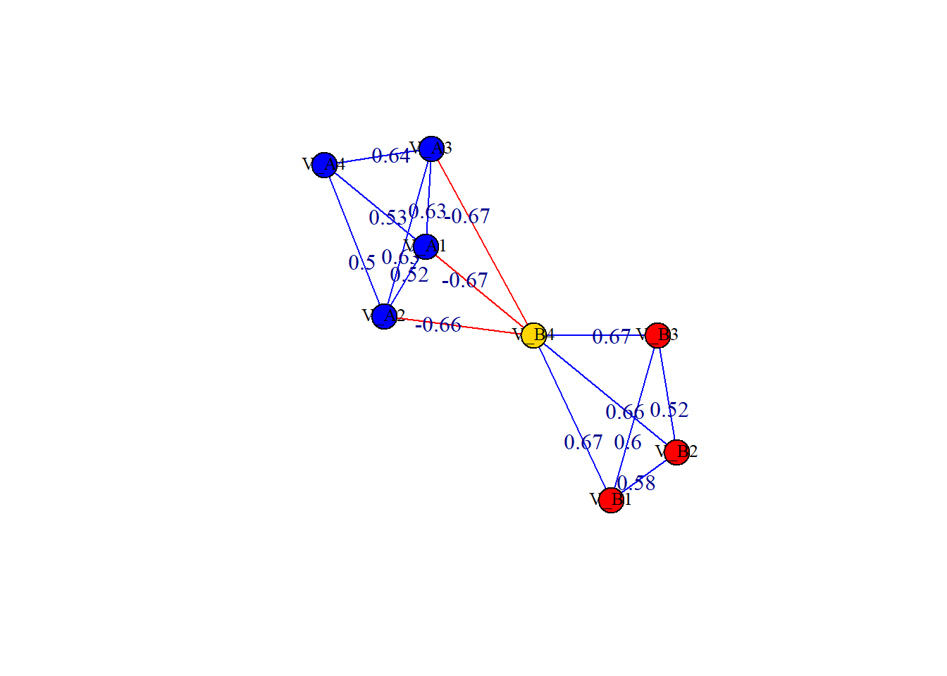

First, we might try to calculate the degree using \(\texttt{R}\). Doing so will yield:

degree(g)

V_A1 V_A2 V_A3 V_A4 V_B1 V_B2 V_B3 V_B4 
   4    4    4    3    3    3    3    6 

Now, that’s a bit strange. The degrees we’re observing are certainly not simply adding up the weighted values. That is because \(\texttt{R}\)–like any computer program–is dumb. From an operational lens, \(\texttt{R}\) is doing the correct procedure: it is adding up the number of links; however, it is ignoring the weights attached to those links.

As we mentioned, degree is renamed to strength. This is also reflected in \(\texttt{igraph}\):

round(strength(g), 2)

V_A1 V_A2 V_A3 V_A4 V_B1 V_B2 V_B3 V_B4 
1.01 1.00 1.23 1.68 1.86 1.76 1.79 0.00 

In the graph, we can calculate the strength for each node. For instance, the strength of \(v_{B3} = 0.67 + 0.52 + 0.60 = 1.79\). Now, degrees and strengths are relative metrics, which implies that they are meaningless without taking into account all other vertices in the graph. Based in our results, \(v_{B3}\) is relatively high in strength compared to the rest of the vertex list.

Note. What other results from this analysis seem curious to you?

Talking Point.

• The strength of \(v_{B4}\) is \(0.00\).

If we were to look at the placement of \(v_{B4}\), one might think that it is one of the most important vertices in the graph as it spans between two highly connected components. However, by the metric of strength, it is essentially, useless. By contrast, its degree is very high.

By merging the two metrics, we see that \(v_{B4}\) is highly connected but that its links sum to \(0.00\).

Throughout the literature, you will find different methods for handling this issue. For instance, in psychological networks, it is common to derive strength as the absolute value of the weighted links. This is because it is a decent compromise. Thus, the strength for weighted, undirected graphs with \(\pm\) links can be calculated as:

\[strength(v) = \sum_{j\in V}|a_{vj}|\]

where–for once–\(|\cdot|\) is the absolute value rather than the cardinality.

Of couse, degree and strength are just one form of definition for importance of vertices in a graph. Next, we move onto the concept of “closeness”.

Closeness

One might think of closeness as a metric which quantifies–on average–how close a vertex is to all other vertices. Thus, a “close” vertex is one that can traverse the graph relatively quickly and connects to other vertices.

Formally, we can define closeness for a graph by:

\[closeness(v) = \frac{1}{\sum_{j\in V} d(j,v)}\] where \(d(j,v)\) is the distance which is conceptualized as the shortest path length between the \(j^{th}\) and \(v^{th}\) vertices. In an undirected graph, the distance would simply be the number of “steps” or links along the most efficient “walk” from one vertex to the next; however, this challenge becomes more complicated with a weighted graph. Bringmann and colleagues (2019) note that–for weighted networks–the distance between any set of vertices may be taken as \(\frac{1}{|e_{ij}|}\) where \(|e_{ij}|\) is the weighted link between the \(i^{th}\) and \(j^{th}\) vertices.

Prior to the \(\texttt{R}\) demonstration, let’s reflect and think about how this definition of closeness may affect the literal translation of distance. Often, in psychology, we are thinking about networks with weighted values that are signed (i.e., \(\pm\)). Using the definition of closeness from Bringmann et al., (2019), we find that \(r = \pm 0.73\) is equivalent for calculating distance. But is that what we intend?

When two variables rise together and are highly positively correlated, is that the same–mechanistically–as two variables with an opposing correlation? What alternative formulations of “distance” would you recommend? Are there any appropriate alternatives?

Preview of Multiplexes.

A toy idea to consider is to generate a “multiplex” graph. Instead of a single graph, imagine 2 graphs which share the same vertices but have unique sets of connections within the layers. We may recast the example posed in the graph \(\texttt{g}\) and re-envision it as a multiplex where each layer is a binary graph comprised of positive connections or negative conncections.

This deals with the conceptual challenge of distance equating \(\pm 1.00\) and–as you’ll see later in the quarter–returns a result that is roughly equivalent to the standard closeness value.

If we were to revisit the graph, \(X = (V, E)\), we could obtain the closeness values for each vertex in \(\texttt{R}\) by:

plot(x)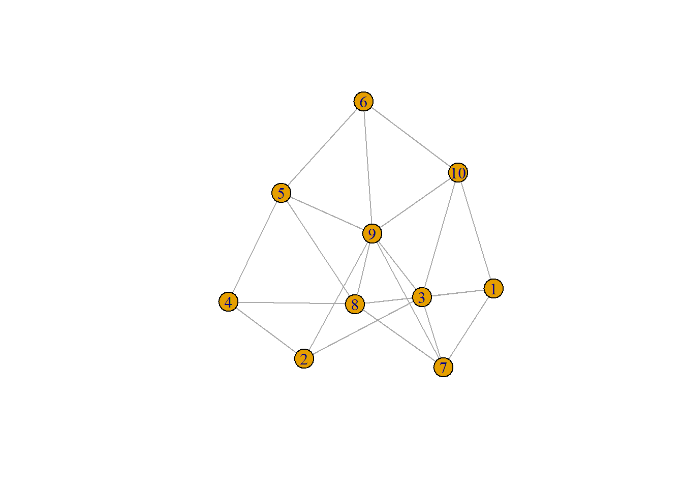

round(closeness(x), 2)

 [1] 0.07 0.07 0.08 0.06 0.07 0.07 0.07 0.08 0.09 0.07

Note that for the graph \(X\), our closeness values are essentially all similar to one another. What might this imply? The conversations related to this will be referenced again later on in today’s lecture.

Betweenness

Finally, we arrive at the betweenness of a vertex. Conceptually, the betweenness describes how often a particular vertex is a mediator between other vertices in the graph. Thus, a vertex with a high betweenness rating may be like a city along a freeway rather than a major destination.

Do note that this is a different idea of “importance” for a node compared to either of the prior definitions we’ve discussed. Consider how these varying definitions–as well as the ones you read this week–may be related to similar or different phenomenon you may be interested in.

We express betweenness as:

\[between(v) = \sum_{v\neq i \neq j} \frac{\sigma_{ij}(v)}{\sigma_{ij}}\] where \(v, i\), and \(j\) are vertices in the set of \(V\), \(\sigma_{ij}\) is the shortest path[s] between the \(i^{th}\) and \(j^{th}\) vertices, and \(\sigma_{ij}(v)\) are the number of shortest paths between \(i\) and \(j\) which involve \(v\) as a mediating vertex.

Thus, betweeness for a vertex will be greater if it is always along the shortest paths but smaller if it is not along the shortest paths.

We can do this in \(\texttt{R}\) using a relatively simple command in \(\texttt{igraph}\) for the graph of \(x\):

betweenness(x)

 [1] 0.8095238 1.1190476 3.5357143 0.8333333 2.1190476 0.6428571 0.2500000
 [8] 5.5119048 7.4285714 1.7500000

When we try to do betweenness on the graph of \(g\), we get an error message:

betweenness(g)

Error in betweenness(g): At vendor/cigraph/src/centrality/betweenness.c:437 : Weight vector must be positive. Invalid value

This is because we cannot have negative weights on our graph. Thus we can use the classic method of taking the absolute value:

g2 = g
E(g2)$weight = abs(E(g2)$weight)
betweenness(g2)

V_A1 V_A2 V_A3 V_A4 V_B1 V_B2 V_B3 V_B4 
   0    4    0    0    0    0    0   12 

In this case, because our graph is weighted, \(\texttt{R}\) uses the weighted form of distance which treats our “correlation” proxy variables as distances. This may or may not make sense for the problem you are working with.

Global Measures

Thus far, the metrics we have discussed are likely familiar to most of the people reading this page. More importantly, each metric has been vertex-specific. That is, they quantify some characteristic of each vertex which we can then compare across vertices to determine the relative importance of one vertex over another. This is all very standard in psychometric networks.

In this following section, we discuss “global” metrics of networks which describe efficiency of influence throughout a network. In these instances, we will obtain a single value which corresponds to some meaningful–we hope–characteristic of the graphs we study.

Density

The density of a graph is a metric describing the ratio of the total number of observed links in a graph relative to the number of possible links. Thus, the formulation of density for a simple undirected graph is quite straightforward and given by:

\[Density = \frac{2|E|}{|V|(|V|- 1)}\]

Where \(|E|\) is the cardinality of our observed edgelist, \(|V|\) is the cardinality of the vertex set and the multiplication by 2 is equivalent to dividing the denominator by 2.

We can make this clearer by understanding that the denominator is just our \(|E|_{max}\). Thus, the undirected simple graph’s density is given by:

\[Density = \frac{|E|}{|E|_{max}}\]

For a digraph with loops, our \(|E|_{max}\) changes. Thus, the equation also does:

\[Density = \frac{|E|}{|V|^{2}}\]

This can be extended to weighted graphs quite simply.

To obtain the densities of graphs in \(\texttt{R}\) we simply call the command:

edge_density(g)

[1] 0.5357143

edge_density(x)

[1] 0.4888889

In psychology, the density of a network has been proposed to be a metric of “inertia” in a similar way that strong positive autocorrelations have are for univariate AR(1) models. Highly connected graphs imply that information–and thereby–influence spreads easily throughout the graph. In contrast, graphs with lower density may be more resilient to certain congation effects.

Alternatively, graphs with less density may be more prone to splitting and breaking apart into smaller components. In psychological systems, this may not seem like a realistic thing that can happen. Thus, we can discuss how density may be relevant for your own substantive interests.

Is connectivity good or bad for various topics you work on?

Average Path Length

The average path length for a graph is given by averging the length of the shortest paths between vertices. We can derive what I will refer to as, \(\bar{PL}\) for a simple undirected graph as:

\[\bar{PL} = \frac{2\cdot\sum_{i\neq j}d(i,j)}{|V|(|V|-1)}\]

Where \(\sum_{i\neq j}d(i,j)\) is the number of all shortest paths between the \(i^{th}\) and \(j^{th}\) vertices repeated across all vertex pairs divided by the total number of possible links, \(|E|_{max}\). Once again, this can be extended to digraphs without self-loops by:

\[\bar{PL} = \frac{\sum_{i\neq j}d(i,j)}{|V|(|V|-1)}\]

In a graph, we can once again use \(\texttt{R}\) to obtain the \(\bar{PL}\) by:

mean_distance(x)

[1] 1.533333

In this case, \(\texttt{igraph}\) is using the weights of the connections in \(x\) as a distance rather than treating the links as binary.

Diameter

Diameter of a graph is a much simpler concept than many of these other metrics we’ve covered thus far because it is quantifying the… well.. diameter of the graph. In this case, the diameter is simply the length of the longest, shortest path. Which may not seem intuitive at first. We can try to explain this concept.

The concept of the “shortest” path is one of efficiency of information travel. Many systems arrange themselves in ways that maximize their efficiency. Likewise, man-made networks such as transportation networks are often build with efficiency in mind because money dictates the degree of inefficiency that is tolerable. Thus, while there may be many ways to traverse through a graph, often, we expect information within a graph to travel efficiently. That is; via the shortest path.

Now, the diameter is given by the “longest, shortest path” and can be derived for an undirected simple graph by:

\[Diameter = \arg\max_{\{i,j\}\in V} d(i,j)\] where the diameter is defined as the maximum distance between an unordered pair, \(\{i,j\}\in V\).

We can express this in \(\texttt{R}\) via the function:

diameter(x)

[1] 3

Now, there are a myriad of other metrics for both local and global descriptions of graphs/networks that we are leaving out. That’s not to say that these other metrics are not important. Rather, it’s that the list could go on indefinitely.

Broadly, I would like to ask you to consider how each of these metrics may or may not align with graphs constructed in your own fields. Is centrality something we might care about? If so, which metrics are more relevant?

Bringmann et al. (2019) discuss the applicability for these centrality indices to networks of psychological constructs. These arguments stem from how information in a psychological network comprised of many symptoms traverses the network. They use examples related to epidemiological and transportation-based systems where efficiency is often maximized deliberately.

Can we make the case that symptoms self-order? Do they take the most efficient route?