gs = list(
  g1 = sample_gnp(n = 10, p = 0.10),
  g2 = sample_gnp(n = 10, p = 0.50),
  g3 = sample_gnp(n = 10, p = 0.90))
par(mfcol = c(1,3))
invisible(lapply(gs, plot))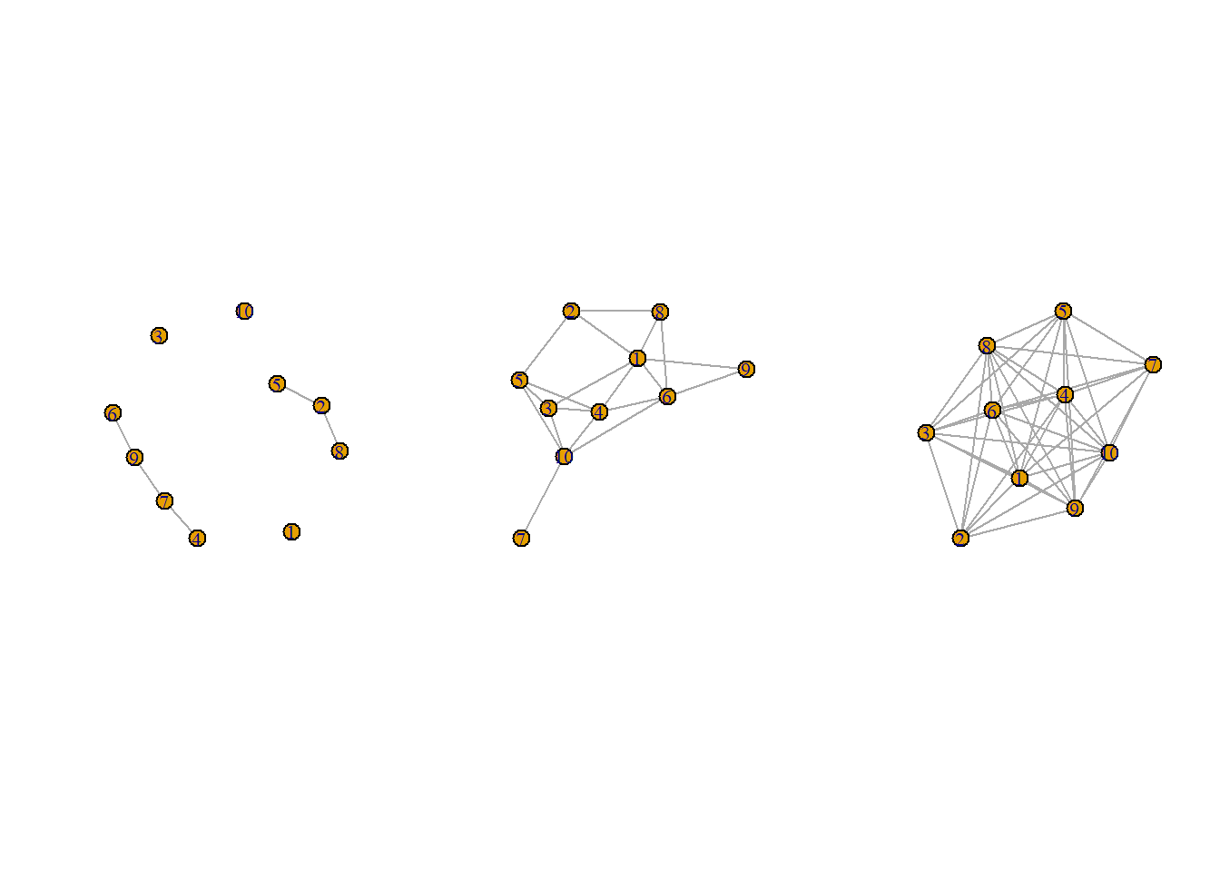
Now, we have discussed different methods for defining the “importance” of certain vertices in a graph. For instance, a vertex of high degree may be highly connected and thus able to exert influence on other vertices. Likewise, a very “between” vertex may be a vital communications pathway between vertices.
Early in our discussion of centrality indices, I mentioned that the importance of a given node is relative to the other vertices. For instance, any arbitrary degree number is meaningless in a vacuum. Thus, knowledge of the graph as whole is vitally important for determining whether a centrality measure is important as well.
To push this idea even further, we can draw on our understanding of basic statistics. For example, a single data point is unremarkable. To obtain a score of 10 could be either fantastic or horrible depending on the scale of measurement and the comparison be they other measurements within or between individuals.
This idea is similar with centrality measures. Their magnitude is comprised both by the substantive data being analyzed but also by the properties of the graph at large. While Bringmann et al. (2019) discussed whether centrality measures were amenable to psychological data, we will–in the section that follows–discuss some of the “forms” graphs can take as a whole and how those forms relate to whether centrality measures can have meaning on an analytical front.
We begin with an exercise. Looking at the graphs below–and given what you read/learned–what about these graphs looks noteworthy? Do you expect the degrees of the vertices in these graphs to differ or be roughly the same? Generally, are the graphs more similar to dissimilar to one another?
Great. Let’s hold our answers in our minds as we progress through the final section of today’s seminar and discuss degree distributions of graphs.
We’ve already discussed how centrality measures are given their importance relative to other vertices in the graphs.
We can solidify this understanding of graphs by characterizing the degree of the prototypical vertex in a graph. For instance, we may be interested in the “average” degree of a graph. If we were to look at the graphs above, we would learn that their average degrees are \(\sim 5.00\).
Hopefully, by knowing the average degree, this leads several of us to ask a deeper question about the nature of the degrees in our graph. Specifically, how are they distributed?
The graphs that we will talk about in the subsequent sections make assumptions on the distribution of vertex degrees in a graph. We will describe how they do so and compound this with a discussion on whether or not degree–and other centrality measures–matter more or less depending on the underlying distribution.
You will find that the idea that centrality measures are distributed in some way is quite understudied in psychology. By contrast, many other fields which use graphs and networks are dominated by literature related to the degree distributions.
The notion that centrality measures may follow some distribution throughout a graph gives rise to questions regarding the downstream effects of these metrics given a distribution.
In some graphs, the vertex with the highest degree may just barely be larger than the degree of other vertices. In those cases, would one feel confident in saying that that particular vertex is influential or important? What about the case when one vertex has an immensely greater degree compared to others?
Does the meaning of degree change in those contexts?
Ultimately, this leads us to the first family of graphs: Erdős–Rényi Random Graph Models.
The Erdős–Rényi random graph model defines a random graph as a distribution of graphs given by 2 parameters: \(n\) and \(p\). Formally as:
\[G(n, p)\]
Here, \(n\) is simply the number of vertices in the graph and \(p\) is the probability of a link between a pair of vertices. Adding from last week, we extend our mathematical terminology by borrowing from combinatorics. For an undirected simple Erdős–Rényi random graph model, we define \(G(n,p)\) where the total possible number of links is:
\[\binom{n}{2} = \frac{n(n-1)}{2} = |E|_{max}\] The first term is read out as, “\(n\) choose 2” and tells us–from the set of vertices–choose 2 to link. We already know it as \(|E|_{max}\). Then, given our \(p\), we can define the expected number of links in our graph as:
\[\mathbb{E}(|E|) = p\cdot\binom{n}{2}\] Given the notation we already know: \[\mathbb{E}(|E|) = p\cdot|E|_{max}\] Thus, for an Erdős–Rényi random graph, we expect the cardinality of our edgelist to be given by \(p\) times the maximum cardinality of the edgelist. The probability that any pair of vertices are selected to share a link is random and uniform.
By contrast, the degree distribution of an Erdős–Rényi random graph is binomial. We can understand the formulation of \(G(n, p)\) as flipping \(n-1\) biased coins. There is a \(p\) probability of heads (a link) and \(1-p\) probability of tails (no link).
Each vertex in \(G(n,p)\) may connect to \(n-1\) vertices with the probability defined by \(p\) giving rise to the following probability mass function:
\[P(\deg(v) = k) = \binom{n-1}{k}p^{k}(1-p)^{n-1-k}\] where \(k \in \{0, 1, \dots, (n-1)\}\)
The expected degree for any random vertex is then given by:
\[\mathbb{E}[\deg(v)] = (n-1)p\] with variance:
\[\mathrm{Var}[\deg(v)] = (n-1)p(1-p)\]
This implies then that the distribution of connections in an Erdős–Rényi random graph are distributed binomially. We might expect degrees of an Erdős–Rényi random graph to be clustered generally around a specific value, \(\mathbb{E}[\deg(v)]\), with variance defined by the binomial distribution.
We may simulate / graphs with a fixed \(n\) and varying \(p\):
gs = list(
g1 = sample_gnp(n = 10, p = 0.10),
g2 = sample_gnp(n = 10, p = 0.50),
g3 = sample_gnp(n = 10, p = 0.90))
par(mfcol = c(1,3))
invisible(lapply(gs, plot))
As you can see, increasing \(p\) increasing the probability of a link between two vertices. We can look at the degrees via:
invisible(lapply(gs, degree))We find that the approximate average degree is given by our expression above, \(\mathbb{E}[\deg(v)] = (n-1)p\). In this case, \(\mathbb{E}[\deg(v)] = (10-1) \times 0.90 \approx 8.10\).
mean(degree(gs[[3]]))[1] 7.4Finally, I no longer have to try to say, “Erdős–Rényi”. Now, we move onto the Watts-Strogatz (WS) random graph model. The historical motivation of the WS random graph is borne out of the Erdős–Rényi random graph and what it couldn’t do.
Namely, real-world networks–as observed by Watts and Strogatz–exhibited local clustering. That is, groups of vertices tended to form cohesive groups with one another. Likewise, graphs formed using Erdős–Rényi fail to exhibit what are referred to as “hubs”. Specifically, vertices with notably higher degrees than others in the graph.
We discuss now how to generate a WS random graph given several defining parameters. Formally, the WS random graph is given by:
\[G_{WS}(n, k, \beta)\]
where \(n\) is \(|V|\), \(k\) is the average degree of the graph, and \(\beta\) represents the rewiring probability for each link. A WS random graph is generated via a ring lattice:
ws1 = sample_smallworld(dim = 1, nei = 2, size = 10, p = 0.00)
plot(ws1)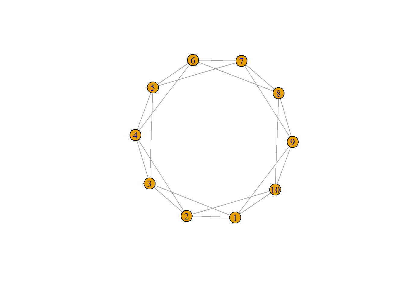
We then “visit” each link in the graph (\(e_{vj} \in E\)) and–given the rewiring probability–assign the link from \(v\) to another randomly selected vertex with the caveat that the newly formed link cannot connect to an already connected vertex or become a self-loop. We observe that by increasing \(p\) in \(\texttt{R}\), we increase the rewiring probability:
ws2 = sample_smallworld(dim = 1, nei = 2, size = 10, p = 0.50)
plot(ws2)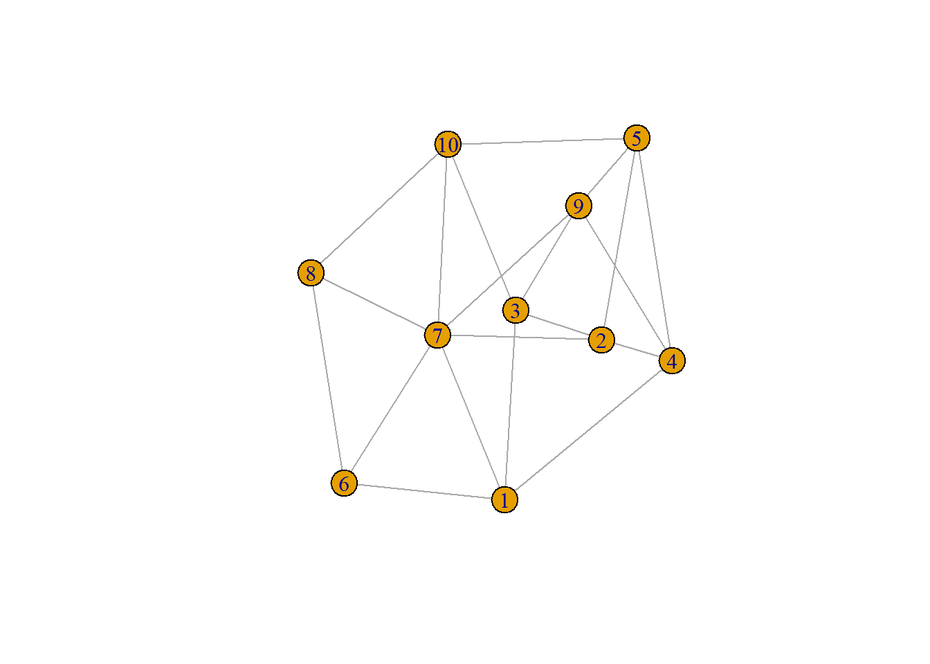
We can assess the properties that result from a WS random graph by simulating a large-scale graph and checking for its asymptotic properties. First, we can start with the \(k\) parameter which corresponds to the average degree. In this case, the \(\texttt{nei}\) argument is \(k = 2\times\mathrm{nei}\)
ws3.1 = sample_smallworld(dim = 1, nei = 1, size = 500, p = 0.20)
ws3.2 = sample_smallworld(dim = 1, nei = 5, size = 500, p = 0.20)
ws3.3 = sample_smallworld(dim = 1, nei = 10, size = 500, p = 0.20)
hist(degree(ws3.1))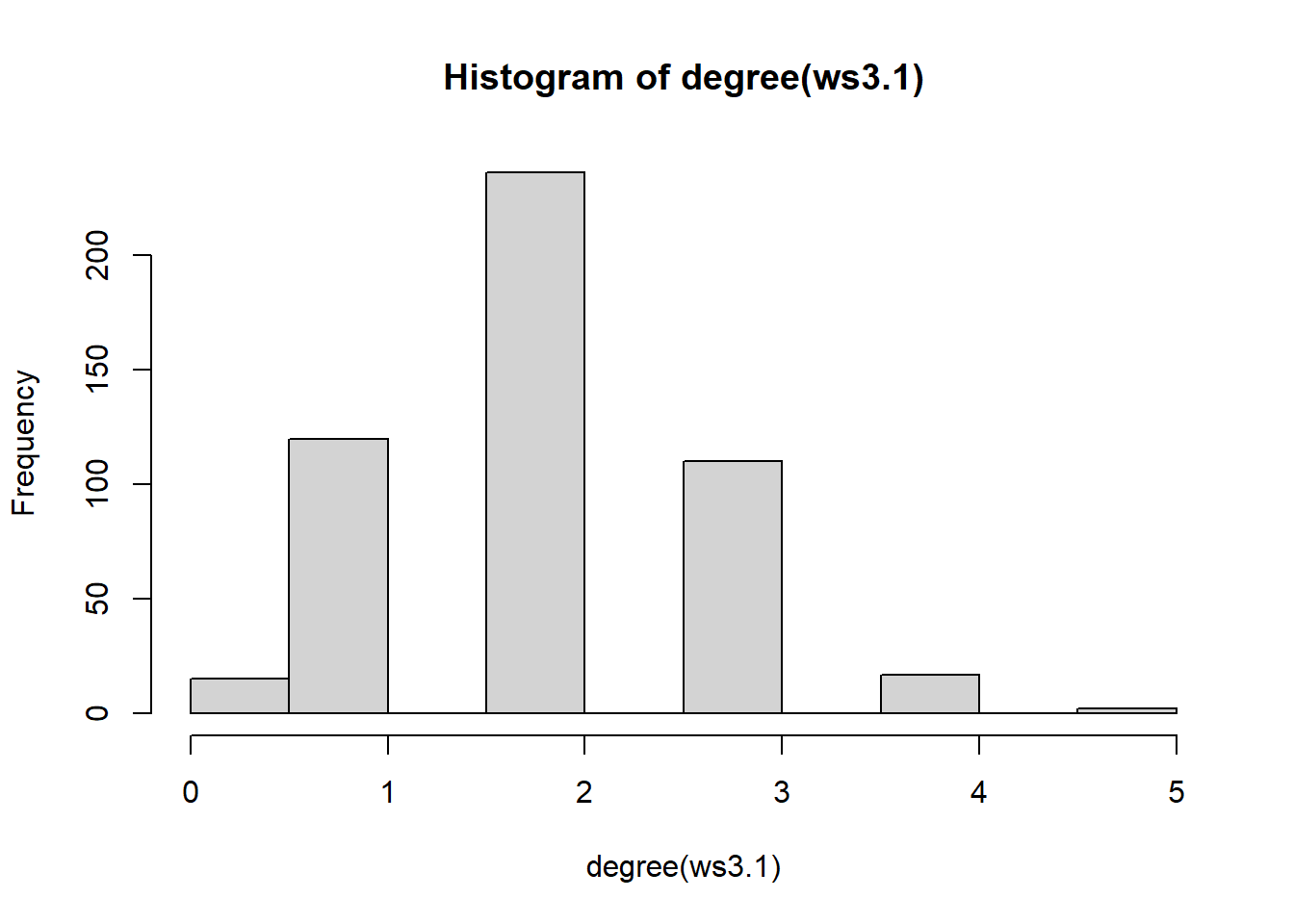
hist(degree(ws3.2))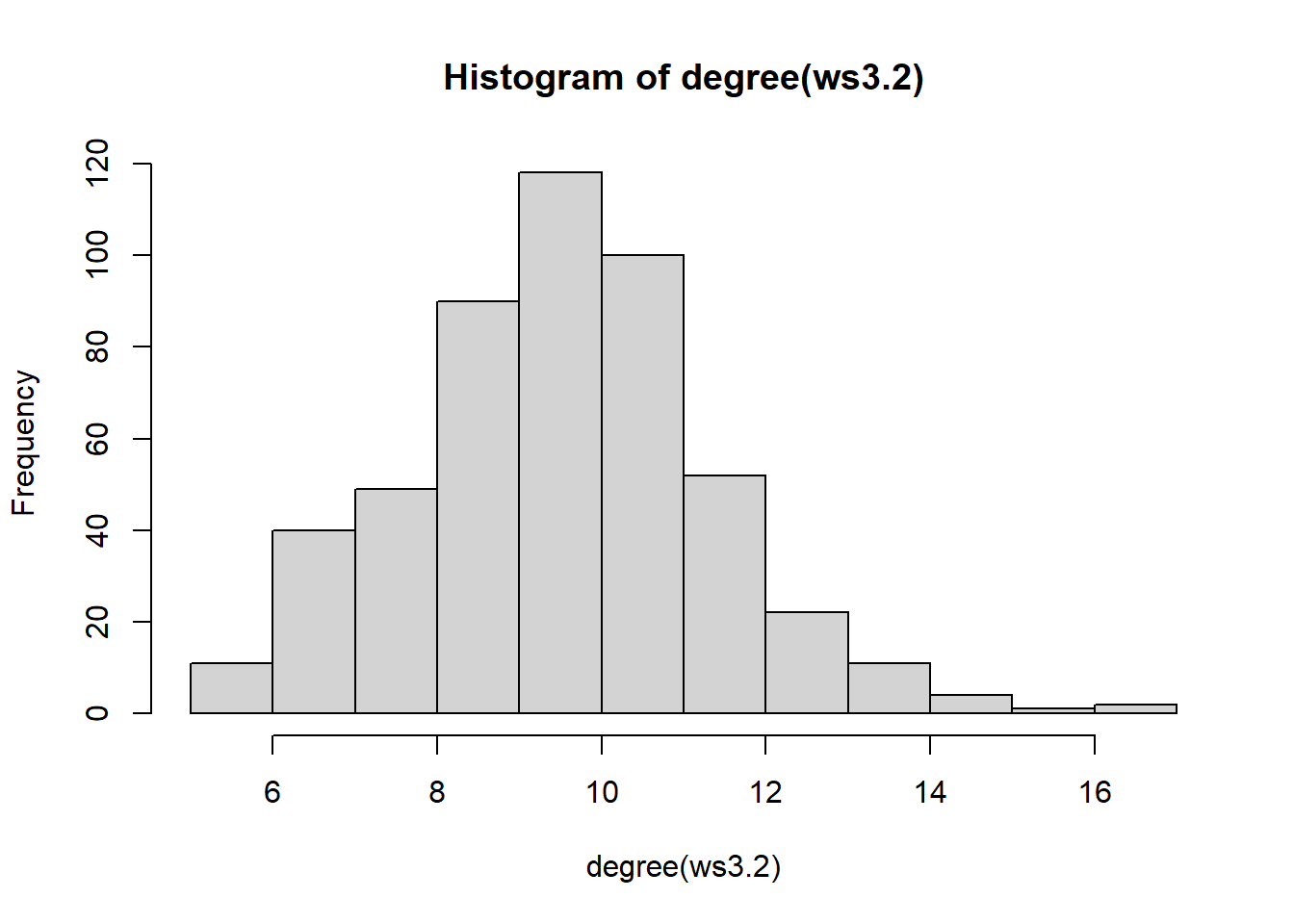
hist(degree(ws3.3))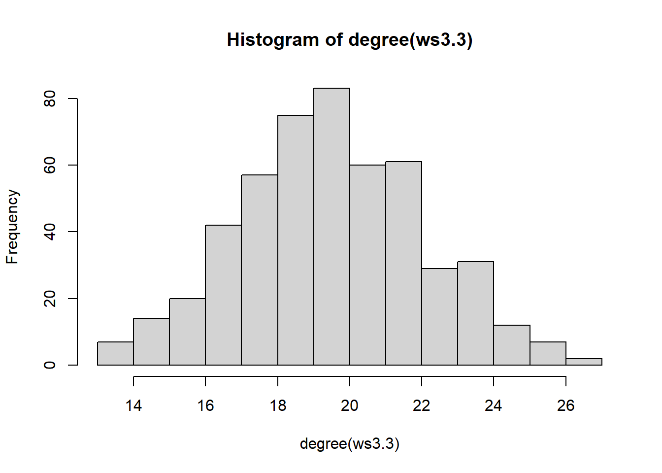
We can also verify the stability of the degree distribution given different rewiring probabilities:
ws3.1 = sample_smallworld(dim = 1, nei = 5, size = 500, p = 0.20)
ws3.2 = sample_smallworld(dim = 1, nei = 5, size = 500, p = 0.50)
ws3.3 = sample_smallworld(dim = 1, nei = 5, size = 500, p = 0.80)
hist(degree(ws3.1))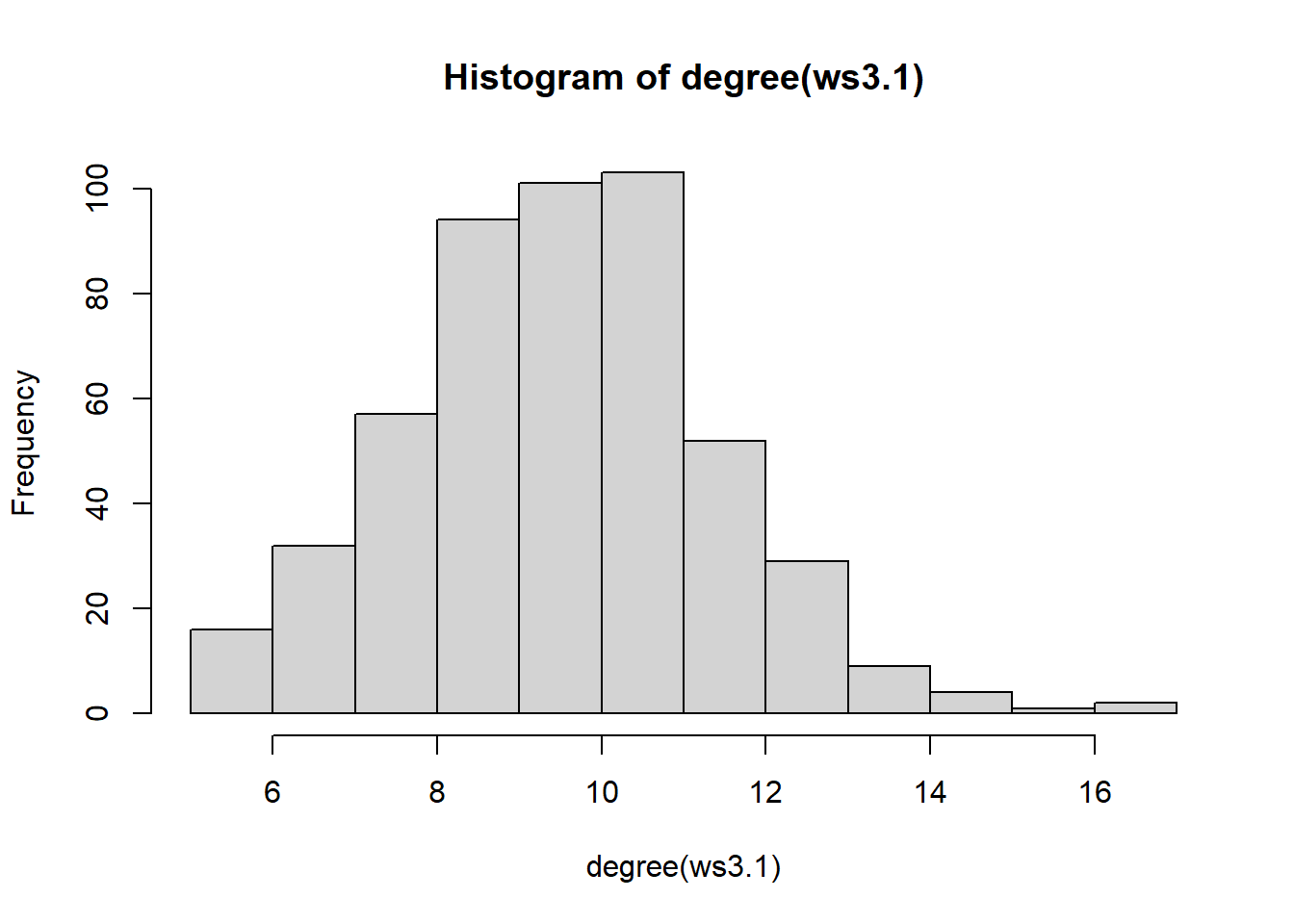
hist(degree(ws3.2))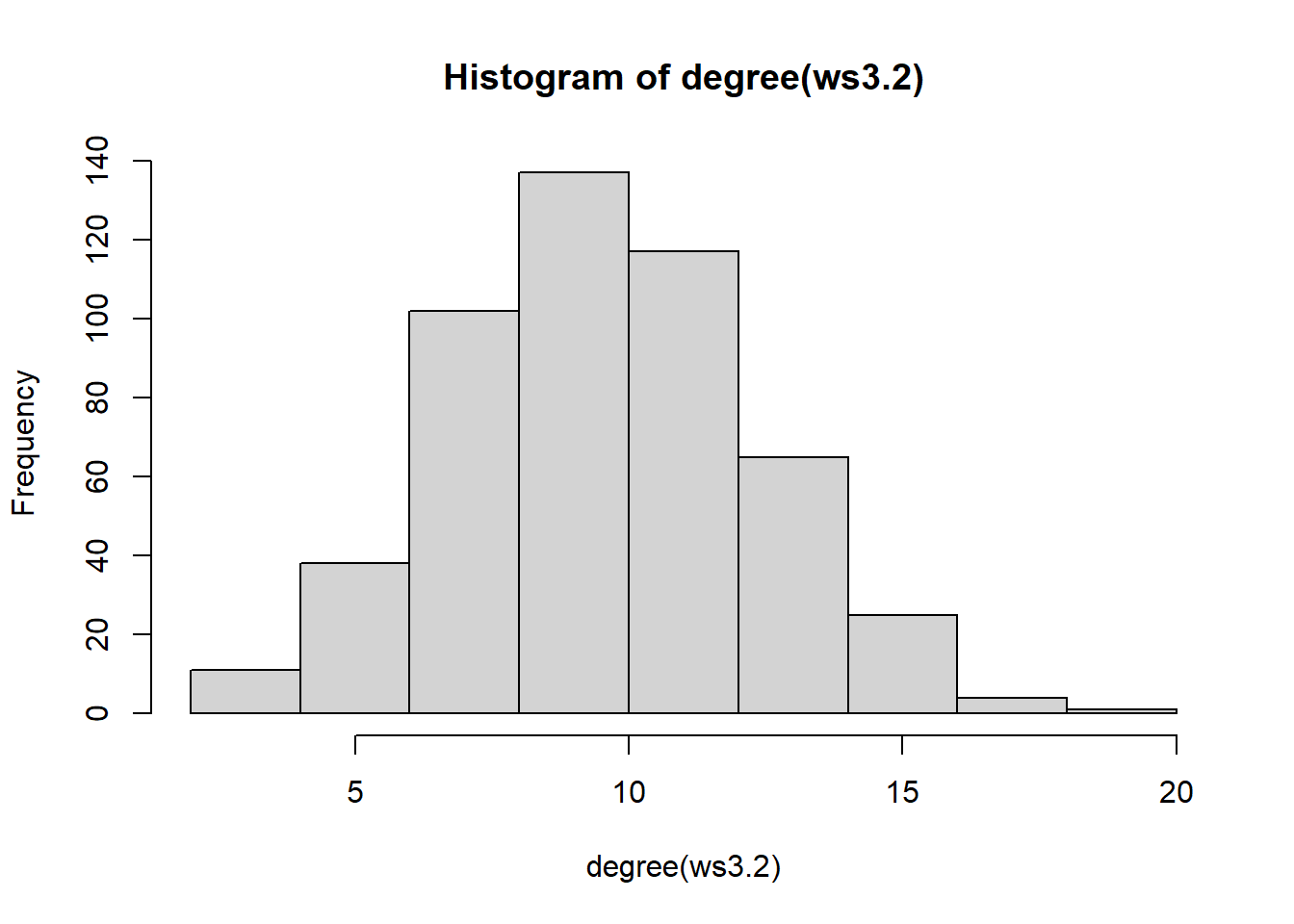
hist(degree(ws3.3))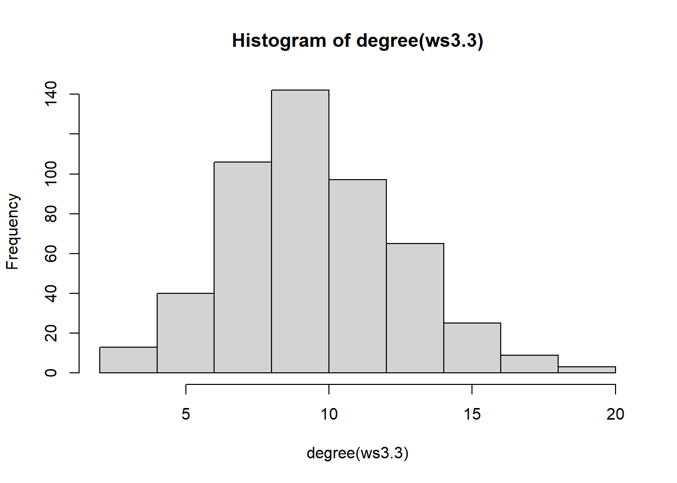
Indicating that the rewiring probability is less related to the average degree or its distribution. The graphs characteristic of WS graphs may often look like they form coherent “clusters” or groups:
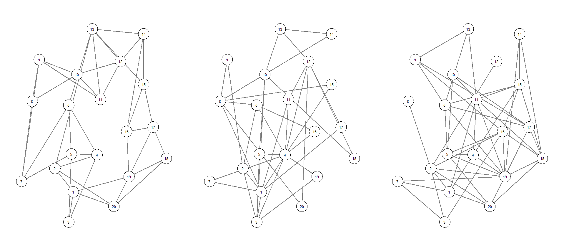
ws3.1 = sample_smallworld(dim = 1, nei = 2, size = 20, p = 0.20)
par(mfcol = c(1, 2))
plot(ws3.1)
plot(ws3.1, layout = layout_in_circle)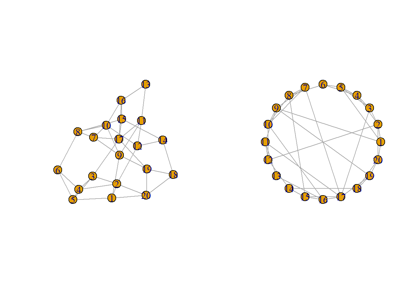
Further, we see how the rewiring affects the graph and its connectivity.
Finally, we arrive at the classic Barabási–Albert (BA) model for random, “scale-free” graphs via preferential attachment. We’ll break down the terms, introduce the model, and discuss–as with the other models–how it generates specific degree distributions.
A scale-free graph is a graph whose degree distribution follows what is known as a “power law”. Formally, this implies that the probability that a randomly chosen vertex has \(k\) links is given by:
\[P(k) \sim k^{-\gamma}\] where \(\gamma\) is a scaling parameter in the range of \(2 < \gamma < 3\) where \(\gamma = 3\) aligns with the “original” BA model. There is an assumption inherent to this idea that the degree follows a power law which is that most vertices have few connections and a small number of vertices have incredibly high connectivity.
The means by which the BA model is generated is via the preferential attachment algorithm. Heuristically, the idea is that you begin with a relatively small graph and add vertices to that graph. Then, links between the newly added vertex are “preferentially” connected based on the existing structure of the graph. This results in a “rich get richer” phenomenon in the graph where vertices with high degree continuously add more links to new vertices relative to less “popular” vertices.
To implement the BA model, we define several parameters:
We begin the BA model by generating \(|v_{0}|\) vertices which are fully connected to one another. At each subsequent step, we add a new vertex and preferentially connect the new vertex to \(l\) existing vertices where \(l \leq |v_{0}|\) to ensure no self-loops or multi-edges.
The probability that the new vertex will connect to the \(i^{th}\) vertex is given by:
\[\prod(i) = \frac{\deg(i)}{\sum_{j}\deg(j)}\] this implies that the probability that the newest \(k^{th}\) vertex links to the \(i^{th}\) vertex is given by how strongly connected it is relative to all other links in the graph. This procedure is then repeated until the graph’s size reaches \(|V|\).
In \(\texttt{R}\), this is done by:
ba.1 = sample_pa(n = 20, power = 1, m = 3, directed = FALSE)
plot(ba.1)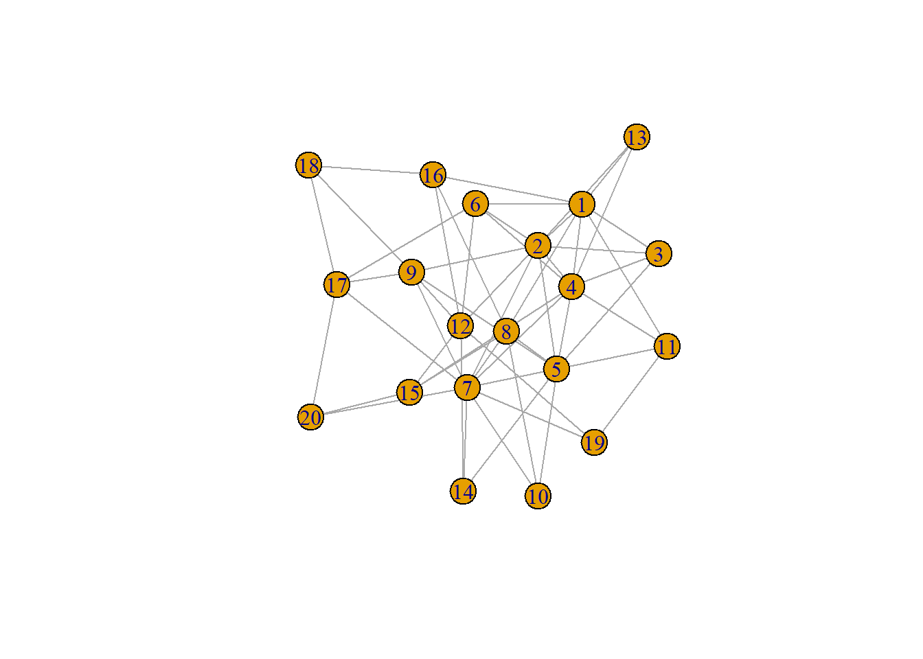
Note that by setting \(\texttt{power = 1}\), we are doing the equivalent to setting \(\gamma = 3\). Smaller values of \(\gamma\) lead to more highly connected vertices whereas higher values lead to fewer.
Many real-world graphs approximately follow power law distributions which is to say that many complex systems self-organize into networks comprised of incredibly connected “hubs” where a majority of vertices are not highly connected.
Social networks are comprised of individuals with very high connectivity while most folks tend to have a handful of close friends. Transportation networks often contain hubs where a signficant amount of travel/traffic passes through whereas many other locales only serve as “sinks” or endpoints of the network.
That said, it is not techincally true that all real-world networks are power laws. Rather, they may approximate power laws or power laws may be the closest approximation but still be pretty bad at describing the observed degree distributions. Ultimately, I have chosen to teach this topic as if power laws accurately describe the real-world networks we encounter very often. Heuristically, it is convenient to say that a heavy-tailed degree distribution is approximately a power law. Just know that this is now always the case.
We close today’s discussion with some questions.
In any of the readings I assigned to you for this week, did you see mention of these various degree distributions? Specifically were these distributions mentioned in any of the articles explicitly related to psychology? You will find that we as a field have generally ignored that the distribution of centrality measures may impact the relevance of these indices as much as the theoretical relevance.
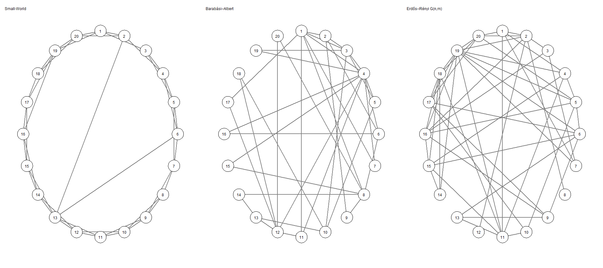
Yet, this topic has remained understudied. We can now revisit the figures I presented at the opening of this topic. Below, we see 3 graphs which appear approximately equivalent to one another.
However, by reorganizing the graph in a circular layout, we see that the graphs–hopefully–look entirely different. By extension, their degree distributions are inherently different because they are a WS random graph, a BA graph, and an ER random graph, respectively.
Let’s touch base on centrality again. Which graph might support the notion that high degree vertices are influential to the function of a graph? Put another way, in which graph would removal of a vertex result in dramatic changes to the topology of the graph? Alternatively, do other graphs seem more or less resilient to the removal of the highest degree vertex? Why?
As noted in lecture, “power laws” despite their popularity and omnipresence in real-world systems, are very rarely power laws. We can make use of some tools for assessing whether an observed degree distribution is likely to have been generated by another known probability distribution. We will do all of this using the \(\texttt{poweRlaw}\) package in \(\texttt{R}\).
We’ll structure these tests around the assumption that many real-world graphs follow power laws. Heuristically, it may be useful to describe a network as following a power law in the sense that a few vertices have most of the links while most others have relatively few. Statistically, it is not the case that many real-world graphs are definitively power laws. Indeed, most of the time, when we are referring to power laws, we are referring heuristically to the tails of the distribution (i.e., heavy tails or a linear trend in a log-log plot). Clauset, Shalizi, and Newman (2009) derived a means to formally test whether an observed degree distribution aligns with any other known degree distribution and I will be providing some sample code for conducting
Recall, a graph whose degree distribution follows a power law exhibits the property that the probability of a vertex possessing a given degree, \(k\) is given by:
\[P(k) = k^{-\gamma}\]
For a continuous power law, we may write the density as:
\[p(k)\mathrm{d}k = \mathrm{Pr}(k \leq K < k + \mathrm{d}k) = Ck^{-\gamma} \mathrm{d}k\] where \(k\) is the observed degree and \(C\) is a normalizing constant defined as:
\[C = (\gamma - 1)k^{-\gamma}_{min}\]
A true power law experiences a divergence as \(k\rightarrow 0.00\) and would render normalization impossible; thus, below a certain value of \(k\), a true power law cannot serve as a valid probability density without a constraint on \(k\) which we refer to as \(k_{min}\). Above \(k_{min}\), one may reasonably expect a power law distribution to emerge whereas below that value, it would unduly affect the recovery of any real power law present in the data.
The method derived by Clauset and colleagues (2009) accepts as inputs the observed degrees of a given graph and attempts to derive a value of \(k_{min}\) where–above that value–a power law may hold. Then, by Maximum Likelihood Estimation (MLE) they attempt to identify the \(\gamma\) parameter of the power law distribution using the identified \(k_{min}\). Finally, bootstrapping can be applied as a form of significance testing to assess the degree to which data were generated from a power law distribution.
We begin by generating data we know come from a power law:
library(poweRlaw)
g.pl = sample_pa(n = 20, power = 1, directed = FALSE)
plot(g.pl)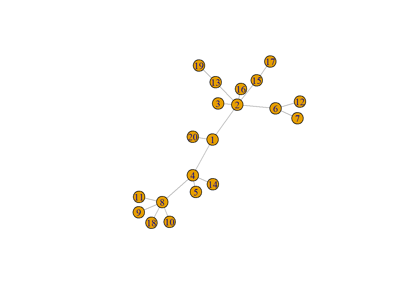
Then, we set up our test:
# Extracting the degrees of our graph
  degrees = degree(g.pl)
# Adding the degrees into a data.frame called "is.powerlaw"
  # The "displ" is saying that our degrees come from a discrete power law distribution [allegedly]
  is.powerlaw = displ$new(degrees)
# This function is estimating the minimum degree. Above which, our data may follow a power law
  is.powerlaw$setXmin(estimate_xmin(is.powerlaw))
# Then, we bootstrap and extract a p-value
  bs = bootstrap_p(is.powerlaw, no_of_sims = 1000, threads = 20)
Expected total run time for 1000 sims, using 20 threads is 0.273 seconds.# The p-value of the boostrap:
bs$p[1] 0.016# The Kolmogorov-Smirnov statistic:
bs$gof[1] 0.1793584Based on the results of the bootstrap method, we see that the data are well approximated by the power law distribution, $p $ 0.016. Here, the null hypothesis is that our data are derived from a power law. Thus a failure to reject the null pushes us to–at the very least–say it’s not… not a power law.
We may do the same for an Erdős–Rényi random graph. Recall, the Erdős–Rényi approximates to a Poisson distribution given a large \(|V|\). Thus, we can test whether the discrete Poisson approximates a graph given by Erdős–Rényi:
set.seed(9103)
g.er = sample_gnp(n = 300, p = 0.40)
Then, we set up our test:
# Extracting the degrees of our graph
  degrees = degree(g.er)
# Adding the degrees into a data.frame called "is.erdosrenyi"
  # The "dispois" is saying that our degrees come from a discrete Poisson distribution [allegedly]
  is.erdosrenyi = dispois$new(degrees)
# This function is estimating the minimum degree. Above which, our data may follow a power law
  is.erdosrenyi$setXmin(estimate_xmin(is.erdosrenyi))
# Then, we bootstrap and extract a p-value
  bs = bootstrap_p(is.erdosrenyi, no_of_sims = 500, threads = 20)
Expected total run time for 500 sims, using 20 threads is 1.41 seconds.# The p-value of the boostrap:
bs$p[1] 0.982# The Kolmogorov-Smirnov statistic:
bs$gof[1] 0.01752282Once again, it appears that the Erdős–Rényi random graph we sampled approximates well. That is, it is not significantly different from a discrete Poisson.
For fun, we can test whether our Erdős–Rényi random graph is different from a power law:
# Extracting the degrees of our graph
  degrees = degree(g.er)
# Adding the degrees into a data.frame called "is.power"
  # The "displ" is saying that our degrees come from a discrete power law distribution [allegedly]
  is.power = displ$new(degrees)
# This function is estimating the minimum degree. Above which, our data may follow a power law
  is.power$setXmin(estimate_xmin(is.power))
# Then, we bootstrap and extract a p-value
  bs = bootstrap_p(is.power, no_of_sims = 500, threads = 20)
Expected total run time for 500 sims, using 20 threads is 14.2 seconds.# The p-value of the boostrap:
bs$p[1] 0.538# The Kolmogorov-Smirnov statistic:
bs$gof[1] 0.102326Based on the results above, it appears that–no–the Erdős–Rényi random graph model is not well described by a power law distribution. Do note, I have tested this in smaller networks and graphs with too few vertices will result in low power.
Finally, we may want to conduct a comparison test to see which of any set of two distributions is likely to have generated an observed degree distribution. We can do so below:
# Describing our graph by Poisson
  g1 = dispois$new(degrees)
  g1$setXmin(estimate_xmin(g1))
# Describing our graph by Power Law
  g2 = displ$new(degrees)
  g2$setXmin(g1$getXmin())
  est2 = estimate_pars(g2)
  g2$setPars(est2$pars)
# Doing the comparison test - Likelihood Ratio
  comp = compare_distributions(g1 , g2)
# Test statistic, R is the LL Ratio
  # Sign indicates which model is better
  # + = first distribution, - = second distribution
  comp$test_statistic
[1] 1007.648# 1-sided p-value provides upper limit on probability of receiving this LL ratio
# If both are equally the same
comp$p_one_sided[1] 0# 2-sided p-value providing probability of getting LL Ratio that deviates in 2 directions
# Provided both distributions are equally good
comp$p_two_sided[1] 0Ultimately, these results would indicate that the graph \(g\)–which we generated from an Erdős–Rényi random graph–are more closely approximated by the discrete Poisson distribution rather than the discrete Power Law distribution.