library(IsingFit)PSC-290: Psychological Networks
Of our previous conversation on SEM (Structural Equation Modeling) and the Latent Variable Model
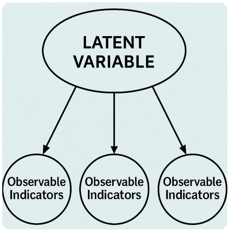
◆ Latent variable model, or CFA (confirmatory factor analysis overall):
For latent variable models:
Assume the latent variable exist -> while in clinical studies it’d be hardly possible to target depression to treat depression.
Assume local independence -> if this is violated and the model exhibits local dependence, then the model fails to capture significant covariance between the items (indicator variables), and leads to biased inference.
There are models attempt to identify local dependence, but they are still problematic in some way, especially since some models do not perform well when the test has limited indicators.
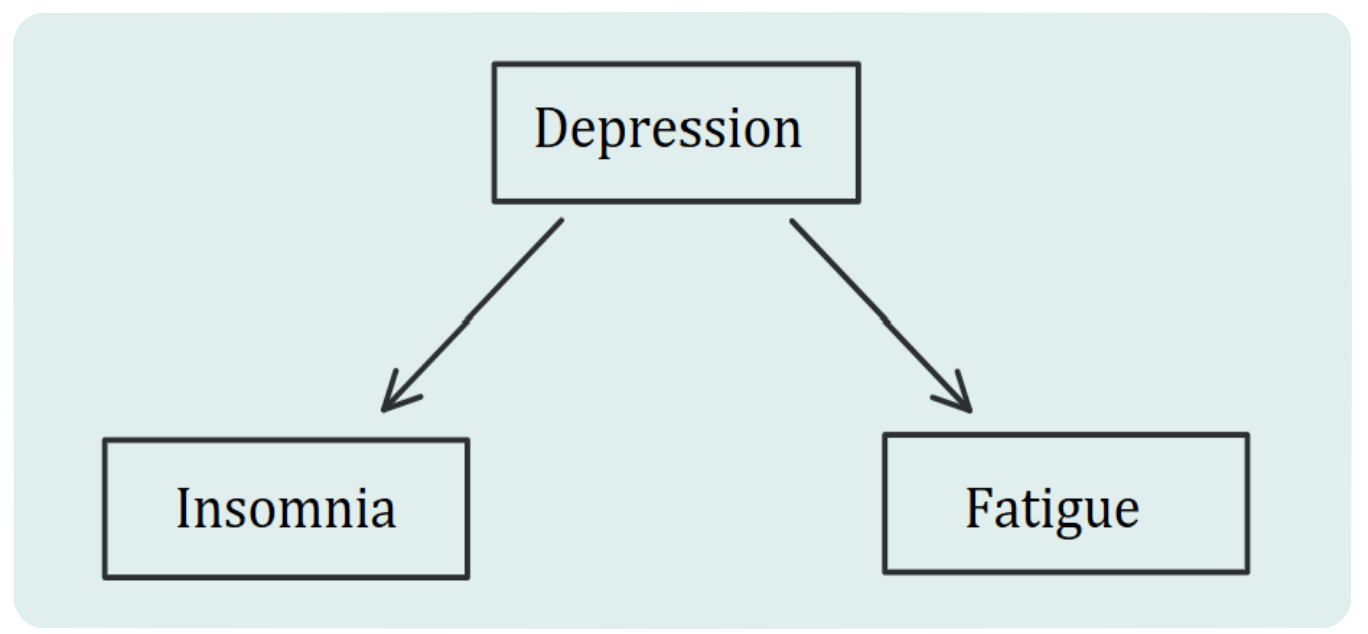
As in clinical level, it’s also anti-intuitive to assume a network of depression that connects insomnia and fatigue, with the indicator variables insomnia and fatigue uncorrelated.
◆ SEM (structural equation modeling)
Here’s the common SEM model:
\[ y_{c} = By_{c} + \Lambda \eta_{c} + \varepsilon_{c} \]
\(\mathbf y_{c}\) : Observed variables.
\(\mathbf B\): Square matrix with zeros on the diagonal of causal effects between observed variables (which the diagonal elements is the variable self-correlation).
\(\Lambda \eta_{c}\): Factor loading matrix for latent variables (represents the relationship between observed variables and the latent factors).
\(\varepsilon_{c}\): Residuals (errors).
So, this is the common SEM equation, allowing us for confirmatory testing of causal models. If you reorder the variables so \(B\) becomes lower-triangular (aka. all zeros above the matrix diagonal), then the system becomes a Directed Acyclic Graph (DAG).
The common reasons to have acyclic structures are:
- The causal interpretation would become ambiguous when a feedback loop occurs in the model. If two factors have a bidirectional relationship, the coefficients would exist in both equations. Therefore, the relationship becomes difficult to interpret.
- Concerns about model stability.
Why do we prefer an acyclic graph?
For DAG, we will have this acyclic directed (recursive) graph that \(A\rightarrow B \rightarrow C\), meaning the graph does not contain cycles (or in a biological sense, a feedback loop like the HPA axis), and thus the edges cannot be tracked from any node back to itself \(A\rightarrow B \rightarrow A\) (non-recursive).
According to Epskamp, even if the repeated measures are at the correct time scale, and adequately model the cycles as acyclic effects unfolding over time, the interpretation could still be problematic.
Therefore, concluding from the two examples above, the reason for adopting the network approach is simple from a biological science or clinical point of view: it represents more of the clinical situation in psychiatry, in which you can say all these symptoms (e.g. excessive anxiety, worry, difficult to control the worry, muscle tension, irritability) are representations of anxiety disorders, but you’ll find it hard to draw a solid line between two symptoms: this one demonstrates anxiety, and this one does not.
Given that, we now move on to psychology networks.
What are Psychology Networks?
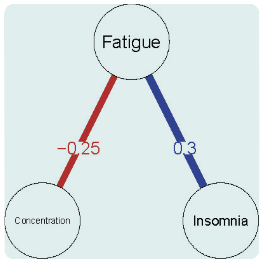
“The network approach has been particularly promising in the field of psychopathology. Within this framework, symptoms (e.g., insomnia, fatigue, and concentration problems) are no longer treated as interchangeable indicators of some latent mental disorder (e.g., depression). Instead, symptoms play an active causal role. For example, insomnia leads to fatigue, fatigue leads to concentration problems, and so forth [Epskamp, 2017]. Psychopathological disorders, then, are not interpreted as the common cause of observed symptoms but rather as emergent behaviors that result from a complex interplay of psychological and biological components.”
◆ Directed Networks
The example in Epskamp’s article above demonstrates a directed network. Yes, since our primary concern for the latent variable model is the debate about the existence of the latent variable itself, how about we just remove the latent variable and keep the causal relation between the factors?
In McNally’s talk at Bath University, he mentioned the Averaged Bayesian Network Analysis:
So instead of one latent variable pointing towards indicators:
We have a causal chain of reactions:
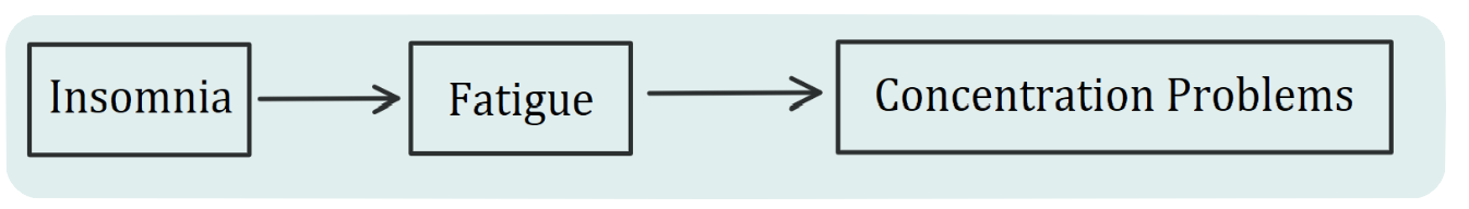
The real-life situation is far more complex than the \(A\rightarrow B \rightarrow C\) shown above, and here is the actual example from McNally’s talk:
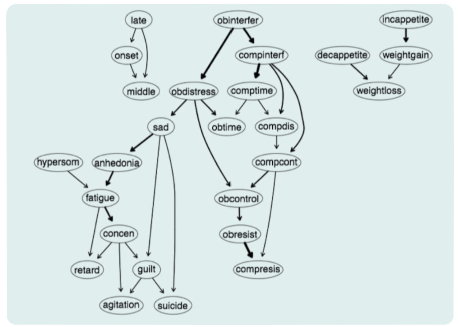
A complex network that allows causal inference, where one factor leads to another. The advantages are clear; this approach allows for causal inference because it’s directed, and one can hope to manipulate the upstream factors to influence downstream chain reactions. Another advantage of Bayesian Networks is that they allow for the prediction of missing data based on the probability of the observed data.
“The connexion between these propositions is not intuitive.” —— Hume
Concerns about unmeasured important variables
Observing X and Y together never proves a necessary arrow, and a hidden Z could generate the conjunction.
Concerns about the candidate causal system
A causal mechanism is defined by (1) a system of physical parts or abstract variables that (2) causally interact in systematically predictable ways so that their operation can be generalized to new situations.
But a basic concern regarding this system is: how is that generalizable causal knowledge possible? “How is it possible to tease apart a target candidate cause’s influence from that due to background causes, in a way that yields causal knowledge that generalizes across the learning and application contexts… the causal invariance constraint: an assumption that there are causes that operate the same way in an application context as in the learning context.” Will future situations resemble the past ones?
Likewise, the Bayesian model assumes the same arrow holds true tomorrow , which he would call an inductive leap.
However, what could be the potential concerns for Bayesian Networks?
◆ Undirected Networks
So, unlike Bayesian networks that use a directed approach, we’re now moving to the undirected networks, which are highly useful in psychological analysis. For those undirected networks, for example, the Markov Random Fields model, the edges between nodes present the potential interactions between the variables, aka. their correlation coefficients. As we dive into our discussion about the Ising model and GGM later today, the Markov Random Fields set the basic structure of those analysis model.
Ising Model
◆ Why should we care about the Ising model?
Simply speaking, the Ising model is a model for pairwise interactions between binary variables, which, is everywhere in psychometrics (presence/absence of an indicator, yes/no insomnia, etc.). And we want conditional relationships like “fatigue predicts concentration problems even after insomnia is present/absent.” And the Ising model offers a transparent way to encode which pairs of variables still matter after controlling for all the others, similar to double dissociation in experimental science.
The Ising Model is originally a mathematical model of ferromagnetism in statistical mechanics named after Ernst Ising and Wilhelm Lenz, used to describe atomic spin interactions. Positive (1) and negative (-1) describe corresponding atomic spins, while the interaction parameters in the Ising model determine the alignment between the variables. For an analogy in psychology, that is: if an interaction parameter (insomnia) between two variables (let’s say concentration problems and fatigue) is positive, the two variables tend to take on the same value (that these two variables are correlated); on the other hand, if the interaction parameter is negative (insomnia absent), the two variables tend to take on different values [Haslbeck, 2020].
Just a distinction between the original Ising model for ferromagnetism and psychology:
Atomic Spin: the domain is { -1, 1 }.
Psychology networks: the domain is { 0, 1}.
Be careful of this domain difference; this would lead to a different interpretation (and we’ll dive into this part later).
◆ eLASSO
Required R Package:
Definition
Let \(x = (x_1,x_2,..., x_n )\) be a configuration where \(x_i = 0/1\). The conditional probability of \(X_j\) given all other nodes \(x_{\setminus j}\) according to the Ising model.
The node-conditional probability of \((x_j)\) given all other variables \((x_{\setminus j})\) is:
\[ \mathbb{P}_{\Theta}\!\bigl(x_j \mid x_{\setminus j}\bigr) \;=\; \frac{\displaystyle \exp\!\Bigl[\tau_j\,x_j + x_j \sum_{k \in V_j} \beta_{jk}\,x_k\Bigr]} {\displaystyle 1 \;+\; \exp\!\Bigl[\tau_j + \sum_{k \in V_j} \beta_{jk}\,x_k\Bigr]}\, \]
where
- \((\tau_j)\) is the node parameter (or threshold) of node \((j)\), which represents the autonomous disposition of the variable \((j)\) to take the value one, regardless of the neighboring variables;
- \((\beta_{jk})\) is the interaction parameter between nodes \((j)\) and \((k)\), which represents the strength of the interaction between variable \(j\) and \(k\);
- \((V_j)\) denotes the set of neighbors of node \((j)\);
- \((x_{\setminus j})\) is the vector of all variables except \((x_j)\).
To obtain sparsity (model parsimony), an \(\ell_1\)-penalty is imposed on the regression coefficients.
L1 Regularization (LASSO)
L1 regularization enhances the model by adding the sum of the “absolute values” of the coefficients as a penalty term to the loss function, promoting sparsity and the selection of relevant features.
L2 Regularization (Ridge)
L2 regularization adds the sum of the “squared values” of the coefficients as the penalty term, encouraging smaller, yet non-zero, coefficients.
Source: Understanding L1 and L2 regularization: techniques for optimized model training | ml-articles – Weights & Biases [Check the article here for more information].
For more about L1 and L2 regularization
A General Overview of the Computing Process:
Randomly select one variable from the set of variables as the dependent variable;
Add an \(\ell_1\)-penalty (LASSO) on all other variables so that the small coefficients shrink to zero to ensure the model is parsimonious;
Choose the tuning parameter with the EBIC ;
Combine the non-zero edges from the p regression (AND-rule or OR-rule).
AND-rule: requires both regression coefficients \(\beta_{jk}\) and \(\beta_{kj}\) to be nonzero.
OR-rule: requires only one of the regression coefficients to be nonzero, and results in more estimated connections.
Visualization.
A Simulation Study | van Borkulo (2014)
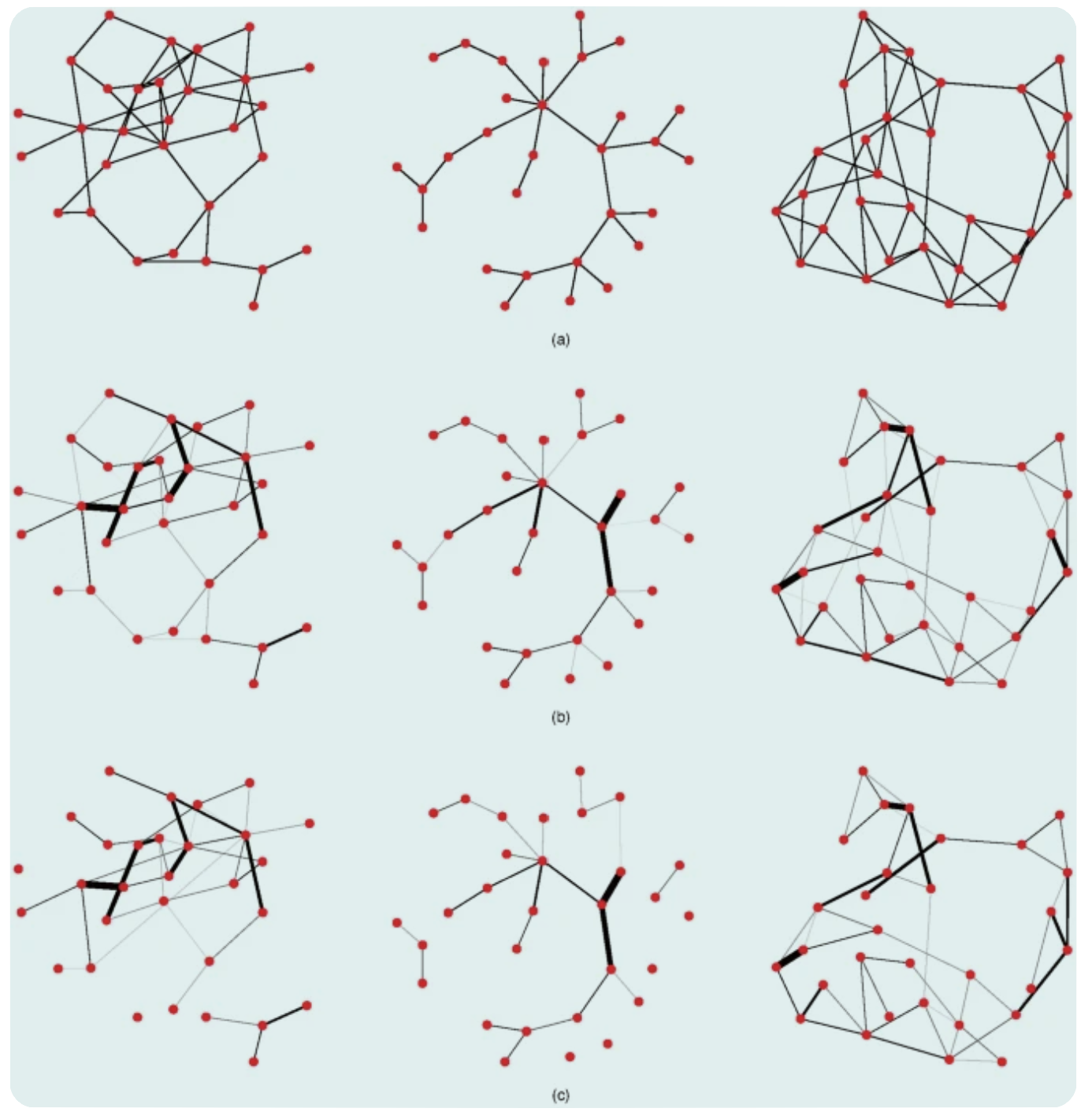
These are examples of networks with 30 nodes in the simulation study.
(a) Generated Networks (from left to right):
random network (the probability of an extra connection is 0.1);
scale-free network (the power of preferential attachment is 1);
small world network (rewiring probability is 0.1).
(b) Weighted versions of (a) that are used to generate data (true networks);
(c) Estimated networks.
From there, we can tell that almost all estimated connections in the true networks are well-represented in the true network (high specificity). However, the weaker connections in the original network are underestimated (low sensitivity).
Exceptions are when the largest random and scale-free networks (100 nodes) are coupled with the highest level of connectivity. In those cases, the estimated coefficients show poor correlation with the coefficients of the generating networks, even for conditions involving 2000 observations. This is because eLasso penalizes variables for having too many connections; therefore, people need to overcome this penalty for networks with larger sample sizes.
[For a real-world example, check the later parts of the report.]
◆ Domain and Interpretation
As we’ve mentioned before, the variables have different domains in psychology and statistics, mechanics networks.
Recap:
Atomic Spin: the domain is { -1, 1 }.
Psychology networks: the domain is { 0, 1 }.
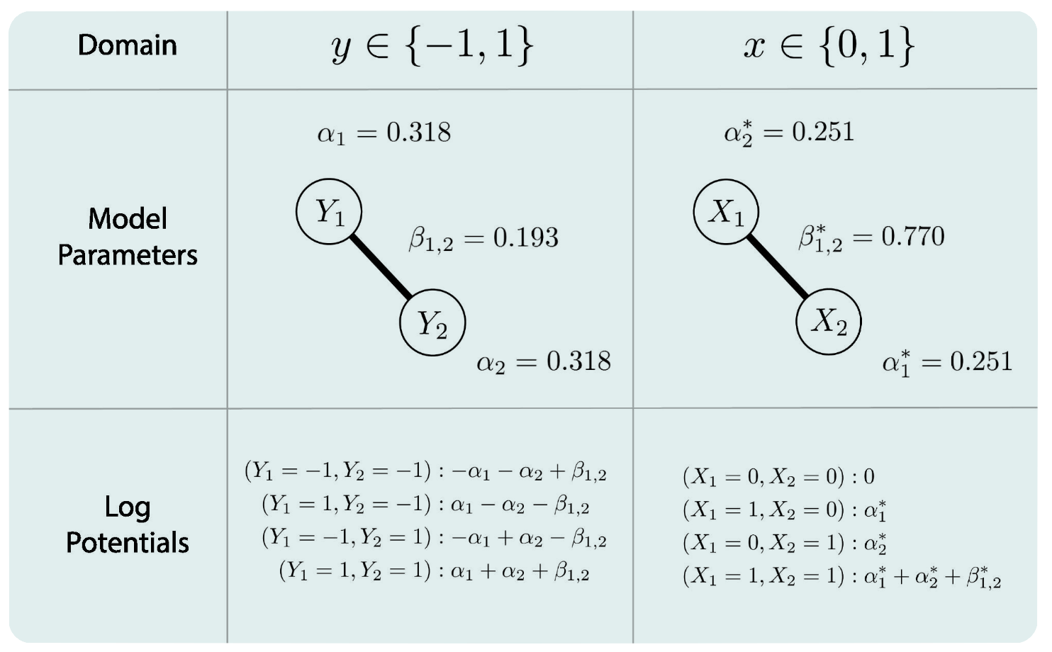
This domain difference will lead to a different interpretation of the result. For a generated model with \(n = 1000\) of the labels \(A, B\), with different domains filled, the obtained parameters are different, leading to various interpretations.
For an Ising model with two variables \((p = 2)\):
\[ P(y_1, y_2)\;=\;\frac{1}{Z}\,\exp\!\bigl\{ \alpha_1\,y_1 \;+\; \alpha_2\,y_2 \;+\; \beta_{12}\,y_1 y_2 \bigr\}, \]
where
\(y_1, y_2\) are either elements of { -1, 1 } or { 0, 1 };
\(P(y_1, y_2)\) is the probability of the event \((y_1, y_2)\);
\(\alpha_1\), \(\alpha_2\), \(\beta_{12}\) are parameters in \(\mathbb{R}\);
\(Z\) is a normalization constant that denotes the sum of the exponent across all possible states. In this case, we have \(2^p = 4\) states.
Regarding those parameters:
\(\beta_{12}\)
Domain { -1, 1 }
For log potentials, if \(\beta_{12}\) becomes larger, then the probability of the states that align { -1, -1 }, { 1, 1 } increases relative to the probability of the states that do not align { -1, 1 }, { 1, -1 }. Alternatively speaking, if \(\beta_{12} > 0\), the same labels align with each other; and if \(\beta_{12} < 0\), the opposite labels align with each other.
Domain { 0, 1 } | What we usually use in psychology networks
When \(\beta_{12}\) increases, the probability of the state { 1, 1 } increases relative to the probability of all other states, and \(\beta_{12}\) models the probability of the state { 1, 1 } only.
\(\alpha, \alpha^*\), when the interaction parameters are allowed to be nonzero:
Domain { -1, 1 }
The threshold parameter indicates the tendency of a variable averaged over all possible states of all other variables.
Domain { 0, 1 }
The threshold parameter indicates the tendency of a variable when all other variables are equal to zero.
Why do we care about the domain?
Communication symmetry: If the author reports the parameter from the { 0, 1} domain, and the reader applies it to the { -1, 1 } domain, they will obtain the incorrect probabilities.
Practical concern: researchers have to choose which version of the Ising model is more appropriate. For example, the { 0, 1 } domain is suitable for values that have situations of “something” versus “nothing”. While the { -1, 1 } domain is helpful to describe whether items are synchronized or not (e.g., positive vs negative affect states, the domain is centered at neutral, 0).
[For more information regarding interpreting the Ising Model, check the original paper here: Haslbeck, 2020]
Gaussian Graphical Model
◆ What is GGM?
Different from the Ising model we just discussed, which captures a network of binary nodes, the Gaussian Graphical Model (GGM) describes pair-wise Markov random fields with continuous data. The GGM estimates a network of partial correlation coefficients, that is, the correlation between two variables after conditioning on all other variables in the data set.
Let’s take a closer look at the formula & definition:
\[ \mathbf{y}_{C}\;\sim\;\mathcal{N}\!\bigl(\mathbf{0},\,\boldsymbol{\Sigma}\bigr) \]
\(\mathbf{y}_{C}\) : Let \(\mathbf{y}_{C}^{\top}= \bigl[\,Y_{C1}\; Y_{C2}\; \dots\; Y_{Cm}\bigr]\)denote a random vector with \(\mathbf{y}_{C}\) as its realization. We assume \(\mathbf{y}_{C}\) is centered and normally distributed.
\(\mathbf{y}_{C}\) can consist of variables relating to one or more subjects, it could also be repeated measures on one or more subjects, or variables of a single subject that do not vary within-subject.
\(\boldsymbol{\Sigma}\): the variance-covariance matrix
But this is not the main focus; in GGM, the graph is determined by the precision matrix \(\mathbf{K}\), which is the inverse of the variance-covariance matrix \(\boldsymbol{\Sigma}\), which \(\mathbf{K} = \boldsymbol{\Sigma}^{-1}.\) Then, the precision network can be standardized to encode partial correlation coefficients of two variables, given all other variables that we have:
\[\operatorname{Cor}(Y_i, Y_j \mid y_{-(i,j)}) = -\frac{\kappa_{ij}}{\sqrt{\kappa_{ii}}\sqrt{\kappa_{jj}}}\]
\(k_{ij}\) is the value from the precision matrix \(\mathbf{K}\) at row \(i\), column \(j\).
\(y_{-(i,j)}\) denotes the set of variables without \(i\) and \(j\).
\(k_{ii}\) and \(k_{jj}\) are the diagonal elements for variables \(i\) and \(j\).
So this gives the partial correlation between variables \(i\) and \(j\), controlling for all other variables. We can therefore represent each variable \(Y_i\) as a node, while having the edges represented by the partial correlation between the two variables.
Here’s an example GGM given in Epskamp’s paper in 2018:
Basically, you have the true variance-covariance matrix first, reverse it (and it becomes a precision matrix); then standardize the precision matrix; there, we have the partial correlation matrix \(R\).
Let’s run a trial with R!
library(GeneNet)
library(qgraph)
library(GGMnonreg)
library(corpcor)set.seed(89181)
# Generating True Model
true.pcor = ggm.simulate.pcor(num.nodes = 10, etaA = 0.40)
# Generating Data From Model
m.sim = ggm.simulate.data(sample.size = 100, true.pcor)# Covariance implied by Data
CovMat = cov(m.sim)
CovMat [,1] [,2] [,3] [,4] [,5] [,6]
[1,] 0.984124544 -0.47187336 -0.2117103 0.13387331 0.03542157 0.50187714
[2,] -0.471873357 0.81644510 0.1467114 0.11954948 0.13728103 -0.20694525
[3,] -0.211710266 0.14671141 0.9243653 -0.20120433 -0.20205149 -0.34530804
[4,] 0.133873309 0.11954948 -0.2012043 1.11213384 0.48538833 0.12258677
[5,] 0.035421567 0.13728103 -0.2020515 0.48538833 0.86230893 0.20832788
[6,] 0.501877139 -0.20694525 -0.3453080 0.12258677 0.20832788 0.94052845
[7,] -0.007323525 -0.09579814 -0.2076763 -0.22158906 0.12845218 0.02472966
[8,] 0.313927735 -0.16870526 -0.6367040 0.17041784 0.37782302 0.58330653
[9,] 0.291349284 -0.09497410 -0.4380250 0.24246617 0.47673171 0.42048845
[10,] -0.079664004 0.17071442 0.1707148 0.09645881 0.09321333 -0.11444492
[,7] [,8] [,9] [,10]
[1,] -0.007323525 0.3139277 0.29134928 -0.07966400
[2,] -0.095798139 -0.1687053 -0.09497410 0.17071442
[3,] -0.207676293 -0.6367040 -0.43802501 0.17071483
[4,] -0.221589057 0.1704178 0.24246617 0.09645881
[5,] 0.128452179 0.3778230 0.47673171 0.09321333
[6,] 0.024729662 0.5833065 0.42048845 -0.11444492
[7,] 1.151495487 0.2663112 0.36488813 0.09466566
[8,] 0.266311175 1.2378489 0.72266048 -0.19123651
[9,] 0.364888131 0.7226605 1.01244217 -0.02390161
[10,] 0.094665660 -0.1912365 -0.02390161 1.03701154# Modeling the true correlations
G1 = qgraph(true.pcor,
bg = "azure2")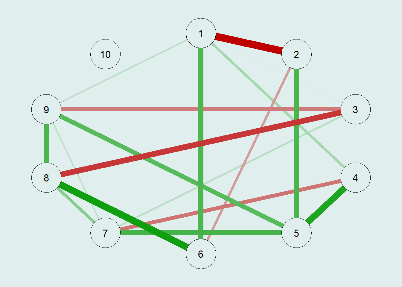
✧ Why do we need model regularization, and what’s the purpose?
Let’s generate the model graphics using the raw precision matrix data:
# raw precision matrix demonstration
pcor.mat <- cor2pcor(CovMat)
G.test = qgraph(pcor.mat,
                bg = "azure2")
So, here we obtain the estimated GGM, which looks similar to the first graph. However, we can see the weights difference, and all the node-pairs are connected, because the raw inverse of the correlation matrix \(\Sigma\) almost never gives exact zeros. Therefore, we need to apply a sparsity-inducing step to ensure our model is as parsimonious as possible. In this case, we’ll use the EBICglasso to reduce the small sampling noises to zero.
◆ Obtaining a sparse network
✧ Extended Bayesian Information Criterion (EBIC)
EBIC is essentially a regularization method that uses LASSO penalty, which helps estimate a sparse GGM by shrinking some connections toward zero. The Graphical LASSO (GLASSO) directly penalizes elements in the inverse covariance matrix without the need for the original variance-covariance matrix. LASSO uses a tuning parameter to find a balance: it can be set to either:
Optimizes cross-validated prediction accuracy, or
Minimize information criteria, like the Extended Bayesian Information Criterion (EBIC) we’re going to discuss.
➣ Why do we use this?
“The EBIC has been shown to lead to the true network when sample size grows and results in a moderately good positive selection rate, but performs distinctly better than other measures in having a low false positive rate.” (van Borkulo, 2014)
Let’s run an EBICglasso Graph:
# Estimating the EBIC Graphical LASSO Network Model
EBICgraph = qgraph(CovMat,
                   graph = "glasso",
                   sampleSize = nrow(m.sim),
                   tuning = 0.5,
                   # penalty for sparsity, another parameter
                   # tuning = 0.0, becomes BIC
                   details = TRUE,
                   bg = "azure2")
In our previous example using the raw precision matrix, the edge was dense, which potentially hides the structural information we truly care about. This EBIC-GLASSO allows us to lower the false positive rate.
✧ Null-hypothesis Significance Testing (NHST)
The NHST is another way to obtain a sparse network by calculating every partial correlation, performing a statistical test, and then dropping insignificant edges.
# Estimating the NHST Gaussian Graphical Model and Generating a Plot
NHSTgraph = ggm_inference(m.sim, alpha = 0.05)
G3 = qgraph(NHSTgraph$wadj)qgraph(G3,
bg = "azure2")
◆ EBIC Regularization Evaluation
Continuing our discussion on EBIC, let’s now move on and test whether it’s a good regularization of our network.
# Calculating the Layout Implied by the 3 graphs
  layout = averageLayout(G1, EBICgraph, G3)
This function allows the node \(i\) to be placed on the exact same spot in all three of these graphs, making it easier for comparison.
# Calculating the maximum edge to scale all others to
  comp.mat = true.pcor
  diag(comp.mat) = 0
  scale = max(comp.mat)
The function above standardizes the network edge widths by the argument “maximum”, so the function is set to the largest absolute weight observed in the true model and makes sure the scaling of the edges is consistent in all three graphs. Also allows easier comparison.
And here’s our graph:
# Creating a Plot
  par(mfrow = c(3, 1))
  qgraph(true.pcor, layout = layout, theme = "colorblind",
         title = "True Graph", maximum = scale,
         edge.labels = round(true.pcor, 2),
         bg = "azure2",
         labels = c("Anxiety", "Depression", "Sleep Issues",
                    ""))
  qgraph(EBICgraph, diag = FALSE,
         layout = layout, theme = "colorblind",
         bg = "azure2",
         title = "LASSO Graph", maximum = scale, edge.labels = TRUE)
  qgraph(NHSTgraph$wadj, layout = layout, theme = "colorblind",
         title = "NHST Graph", maximum = scale,
         bg = "azure2",
         edge.labels = round(NHSTgraph$wadj, 2))
# Asessing the fit of the EBIC LASSO Regularized Network
  ggmFit(EBICgraph, CovMat, nrow(m.sim))
ggmFit object:
 Use plot(object) to plot the network structure
 Fit measures stored under object$fitMeasures

             Measure    Value
1               nvar       10
2               nobs       55
3               npar       24
4                 df       31
5               fmin     0.17
6              chisq    34.81
7             pvalue     0.29
8     baseline.chisq   314.97
9        baseline.df       45
10   baseline.pvalue < 0.0001
11               nfi     0.89
12               tli     0.98
13               rfi     0.84
14               ifi     0.99
15               rni     0.99
16               cfi     0.99
17             rmsea    0.035
18    rmsea.ci.lower        0
19    rmsea.ci.upper    0.085
20      rmsea.pvalue     0.63
21               rmr    0.065
22              srmr    0.068
23              logl -1273.96
24 unrestricted.logl -1256.56
25            aic.ll  2595.92
26           aic.ll2  2611.92
27             aic.x   -27.19
28            aic.x2    82.81
29               bic  2658.44
30              bic2  2582.65
31              ebic  2768.97
32        ebicTuning     0.50
From our demonstration above, we can then see that the EBIC-glasso recovered the overall topology well (the significant edges included in the NHST Graph are well represented in our LASSO Graph). However, even after taking into account sparsity, the density of connections still faces the risk of over-estimation (but we can also use a slightly larger EBIC tuning parameter for a clearer graph).
Below is the code for a network comparison test:
# Network Comparison Test
  library(NetworkComparisonTest)
  true.pcor1 = ggm.simulate.pcor(num.nodes = 10, etaA = 0.20)
  true.pcor2 = ggm.simulate.pcor(num.nodes = 10, etaA = 0.50)
  m.sim1 = ggm.simulate.data(sample.size = 100, true.pcor1)
  m.sim2 = ggm.simulate.data(sample.size = 100, true.pcor2)
# Elaborating on options and results; in this case, networks differ:
# In structure but not in global strength
nc.test = NCT(m.sim1, m.sim2, it = 2000)readRDS("./result.RDS")
 NETWORK INVARIANCE TEST
 Test statistic M:
 0.684136
 p-value 0.0004997501

 GLOBAL STRENGTH INVARIANCE TEST
 Global strength per group:  5.432409 1.71551
 Test statistic S:  3.716898
 p-value 0.0004997501
◆ Model Interpretation
Predictive Utility
GGM can be interpreted without any causal interpretation, and it’s a great tool to show which variables predict one another. So instead of \(A \rightarrow B \rightarrow C\), we have \(A-B-C\), and only the node \(B\) is needed to predict \(A\) or \(C\) — a great tool to map out multicollinearity.
Indicative of Causal Pathways
The GGM is closely tied to causal modeling, so instead of “proving” a causal relationship, it’s indicative of potential pathways. An edge \(A-B\) could exist may maybe due to a causal link between the variables (\(A \rightarrow B\) or \(B \rightarrow A\) ). Since GGM is an undirected network, it doesn’t suffer from acyclicity and does not feature equivalent models. Therefore, edges in the GGM may be interpreted as indicative of potential causal pathways (but be careful about the wordings here, and we’ll discuss them later in this discussion).
Causal Generative Models
Undirected network models were being used as data-generating models, which allows for a unique causal interpretation: one of genuine symmetric effects.
A Discussion | Does regularization align with our conceptual understanding of real-world psychological networks?
◆ The Debate of Sparsity
As we discussed earlier in the Ising model and GGM, we always assume the true network to be sparse, meaning that we assume the true structure can be simplified in some way, because otherwise, too many observations are needed to estimate the network structure.
However, is that really the case? Can our truth be not sparse, but dense in nature?
Here, Epskamp et al. ran this test to estimates an Ising model when the truth is dense:
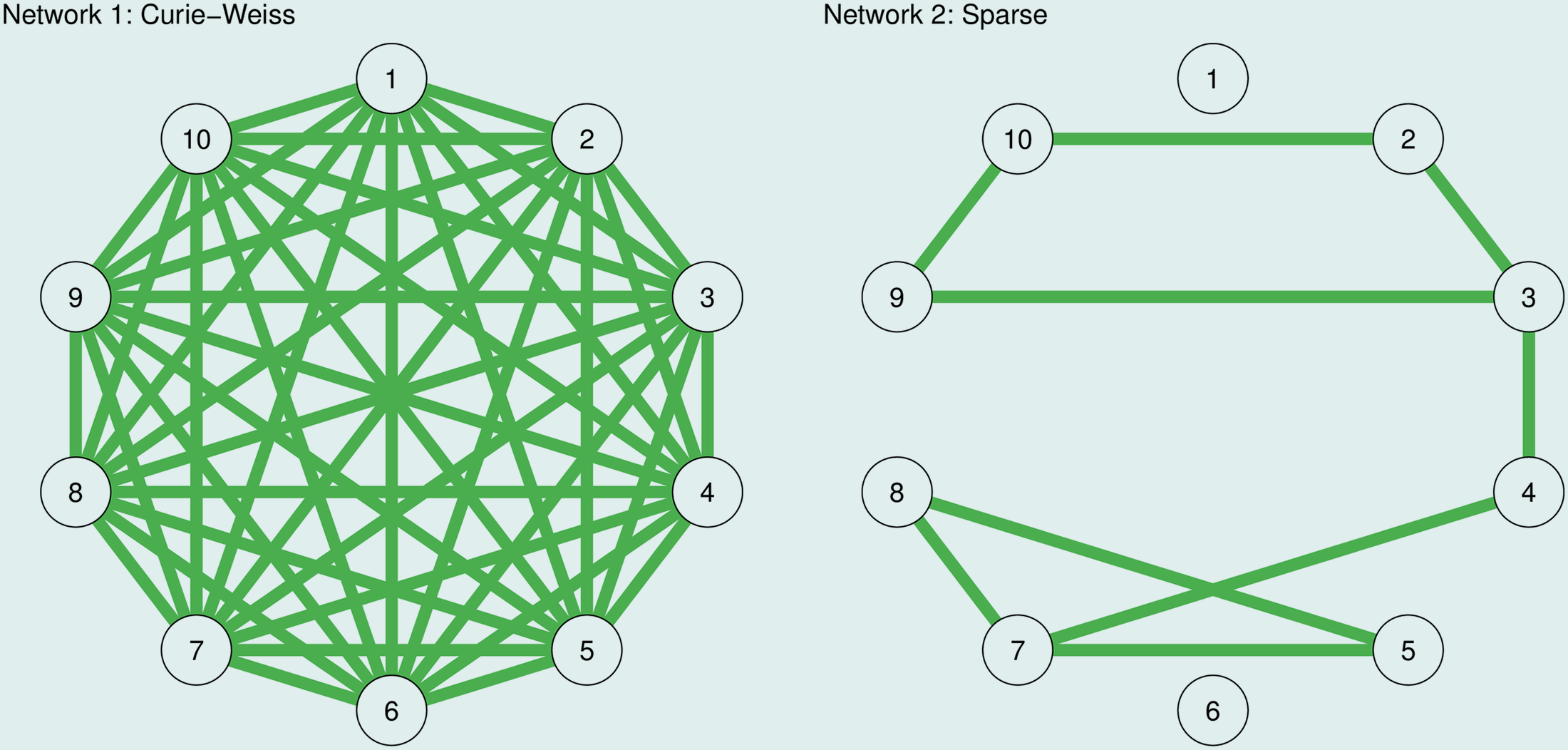
So they simulated 1000 observations from the true models in the image above. The Curie-Weiss model is fully connected, and all edges have the same strength (here set to 0.2). And the second model on the right is a sparse network in which 20% of randomly chosen edge strengths are set to 0.2, and in which the remaining edge strengths are set to 0 (no edge).
And below are the simulation results:
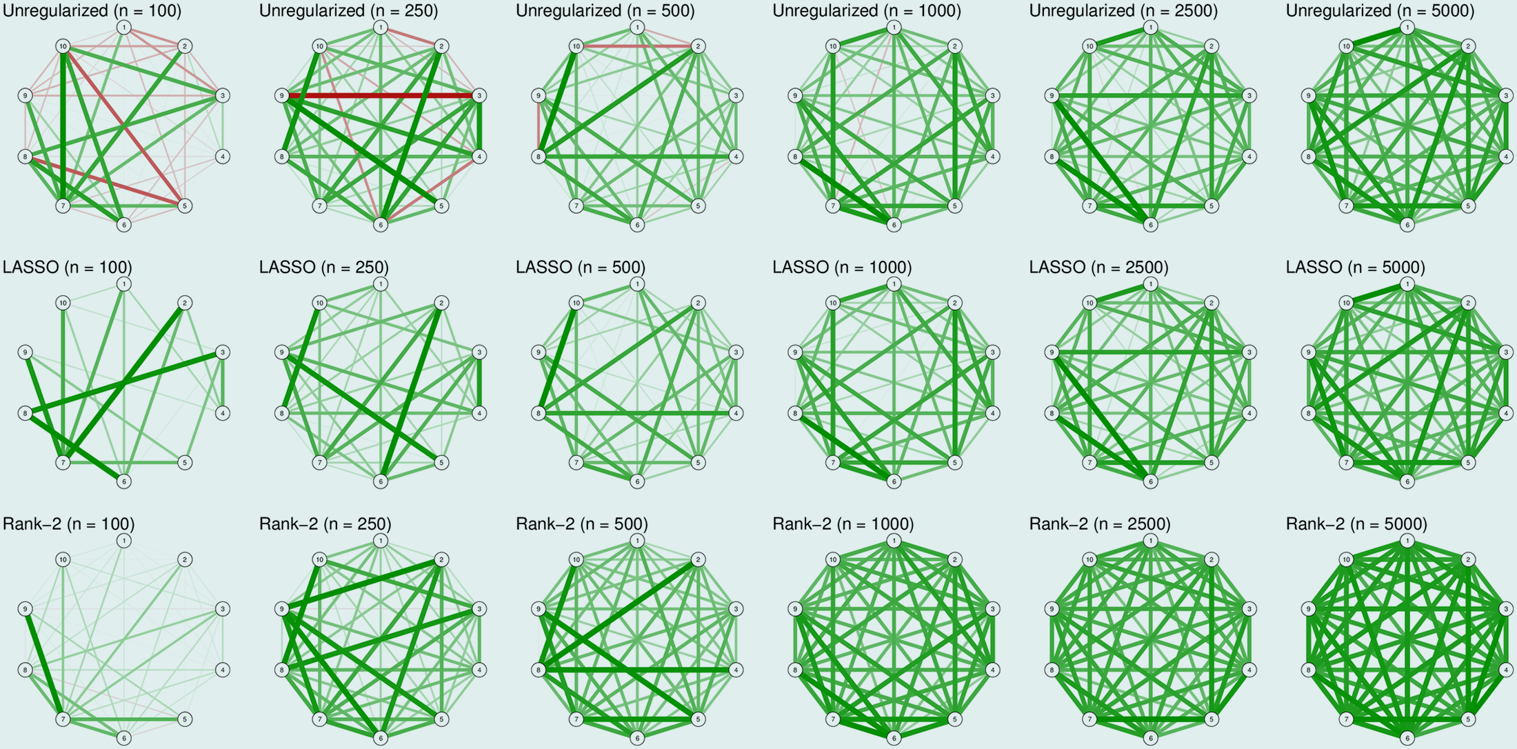
In Rank-2 approximation, the matrix is composed of two latent dimensions, similar to two-factor model.
In case you’re not familiar with rank-2 approximation.
From our demonstration above, the unregularized network for the first true model captured a number of spurious differences in edge strength, including many negative ones. Though LASSO estimation seems a better option, it still does not capture the true model (since it suppresses sparsity). In this case, when the true network is dense, a rank-2 approximation seems to work best in capturing the model. But as the sample sizes increase, all methods perform well in capturing the true model.
Moving on to the second true model (sparse):
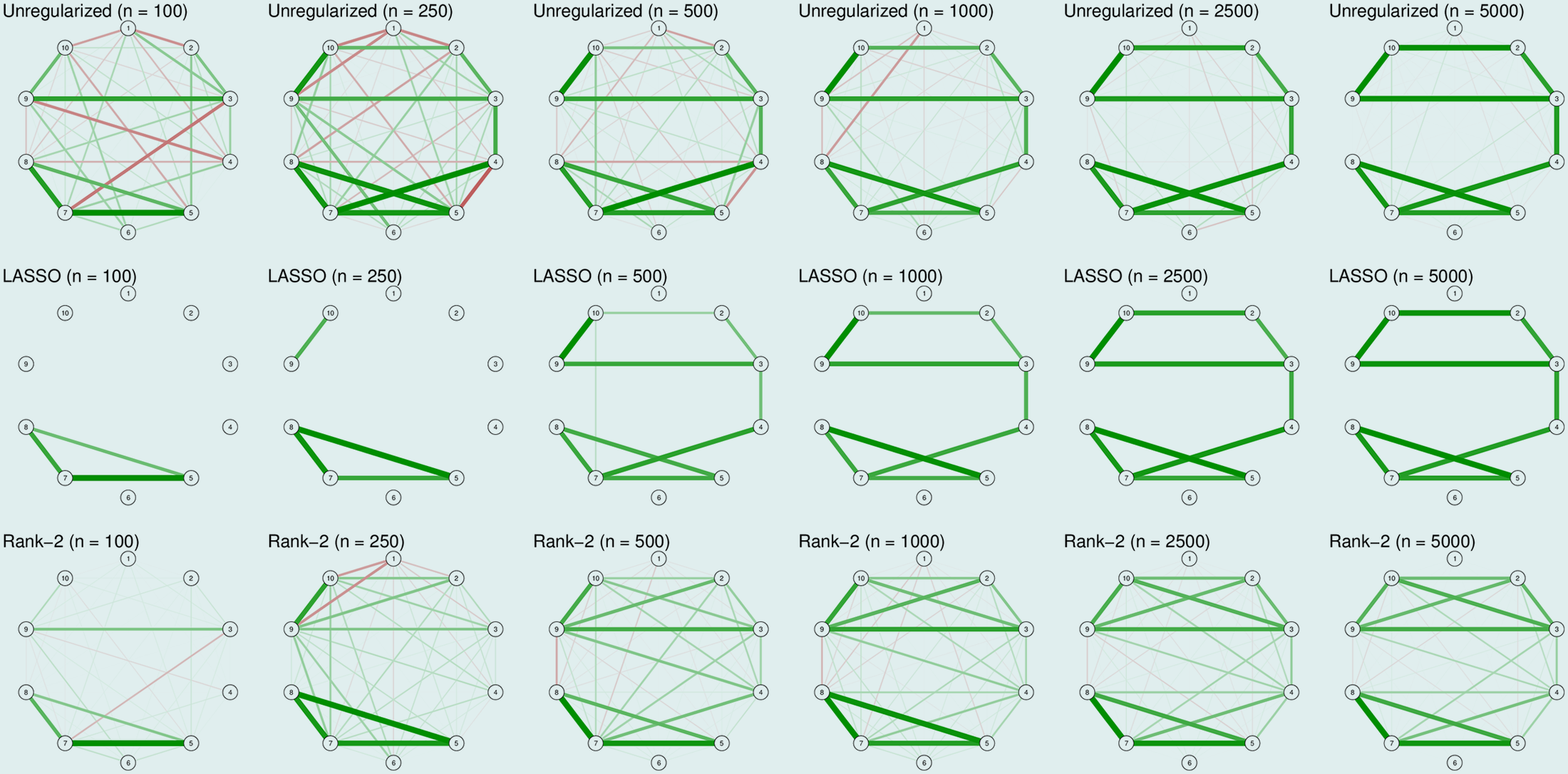
There we see that LASSO is doing its work here, performing great capturing the true structures. In comparison, rank-2 approximation has a poor specificity even with a large sample size of 5000.
Therefore, this shows that the LASSO and low-rank approximation only work well when the assumptions on the true underlying model are met.
◆ Of the Assumed Symmetry of the Correlation Matrix
I’d like to discuss this topic because the mismatch between the model assumption and the real-life situation has always made me wonder: Does the correlation matrix, with its diagonal symmetry, truly represent the psychological processes?
Indeed, mathematically speaking, the covariance between two nodes is symmetric. This correlation matrix symmetry is what we assumed in factor models and basic network models, given that:
\[ cor(A, B) = cor(B,A) \]
And we naturally interpret, say \(A\) means insomnia and \(B\) means fatigue:
The correlation between insomnia \(\rightarrow\) fatigue (\(A\rightarrow B\)) is, say, 0.3,
And the correlation between fatigue \(\rightarrow\) insomnia (\(B\rightarrow A\)) is also 0.3.
This assumption is so natural that it’s built on the math of Pearson correlation coefficient, and does not capture directionality, therefore treating the relationship as bidirectional and symmetrical by default.
But how would you interpret this covariance? If someone aims to take a causal inference, again, take the depression network for example, the node “insomnia” and node “fatigue” demonstrate a covariance of 0.3, does that mean their interaction is equal and has a magnitude of about 30% of one unit change?
In other words, in real-life situations, asymmetrical causal influence is very common. We have so many nodes/symptoms pointing to fatigue, making it a common endpoint and not directing anywhere else; meanwhile, insomnia is targeting a bunch of other symptoms and triggering a chain reaction, etc. What information can we get from this covariance relation, and what kind of conclusion can we draw from the study?
◆ Of the Interpretation of Psychological Networks
As we’ve just discussed, the psychological networks may not necessarily have symmetrical correlations, making our interpretation of the correlation difficult. And here we are facing another interpretation problem:
If those elements (nodes) are significantly connected (by edges), what can we take from that information?
Below are several related thoughts on psychological networks, just to initiate the conversation & discussion.
✧ Two Competing Theories: The Latent Variable and Network Models
As we’ve mentioned in the first part of our discussion, the Latent Variable Model assumes the existence of a latent variable that is causing all the symptoms; and the Network Model suggests a bunch of nodes that are connected by edges. But just think about this question: how do we define a node?
Just like we used to believe autism and Asperger’s are two separate diagnoses, now we think those fall on different parts of the Autism Spectrum Disorder (ASD). How do we know two seemingly unrelated disorders are related in some way?
“When studying co-morbidity based on diagnoses, this inevitably leads to the question of what we actually observe when two disorders covary: genuine covariation between two real disorders, or covariation between certain constellations of symptoms we have designated to be disorders, but that are in fact not indicators of the same latent variable?” [Humphry and McGrane, 2010]
In DSM-V Substance Use Disorder, the diagnostic criteria state:
[1] Taking the substance in larger amounts or for longer than you’re meant to
[8] Using substances again and again, even when it puts you in danger
[10] Needing more of the substance to get the effect you want (tolerance)
If you are familiar with pharmacology, you’d know all of these is pointing to the same terminology “tolerance”. Then, in a sense, if we find some correlation with these three criteria, could it just mean that the patient is building tolerance, essentially a latent variable? And if we think this further, we trace down to the neurological, chemical, and physical mechanisms, does the distinct boundary between variables even exist?
But eventually, we allow ambiguity. This is also where statistics chime in, and we gladly take the 5% risk that the phenomenon is just a false positive.
Think a bit before you click: About the boundaries between variables.
✧ A thought on network causal inference
“The important message here is that models with excellent fit tell us little about the data generating mechanism due to statistical equivalence. A well-fitting factor model cannot be taken as evidence or proof that a psychological construct such as the p factor or g factor exists as a psychological construct (Kovacs & Conway, 2019; Vaidyanathan et al., 2015; van Bork et al., 2017). Similarly, a network model with good fit to the data cannot tell us where we need to intervene in a causal system—e.g., on x3 in Figure 2, which has the highest centrality (i.e., interconnectivity, operationalized as sum of all connecting edges)—because the data may have been generated under an alternative causal model such as the common cause model, in which case intervening on x3 would not change the other variables because they are independent given the common cause.” [Fried, 2021]
Though I mentioned GGM is a good tool to indicate potential causal links between nodes, that’s still limited to an exploratory approach, and it eventually does not “prove” that the causal relationship actually exists. A node that is highly correlated to many other nodes could just be a common outcome, for example, many diseases and disorders can lead to fatigue, but is that helpful, in a pharmacological sense, that we can manipulate the level of fatigue and trace back to the chain reaction, and make a change at upper-stream variables?
Adding to that, even though viewing from a psychological level, it seems there are no hidden nodes between insomnia and fatigue, but if we think of it at a biological level? Circadian rhythms? Signaling pathways?
✧ Non-uniformity of Psychological Disorders
“Our depressions seem to be different.”
Similar to our case in the previous discussion about node definition, how we define the network (or the psychiatric disorder itself) is also an unresolved question.
Or, we could put the question in another way: Is there an essence of, say, MDD, just like how the presence of an extra \(21^{st}\) chromosome defines Down’s syndrome?
✧ Other Concerns
In the article What Do Centrality Measures Measure in Psychological Networks, the authors raised another question regarding the network flow. Simply speaking, they introduced three main flow processes:
Parallel: can be captured with degree/closeness centrality (e.g., email network & virus sent out, as emails spread through the network simultaneously, every vertex linking to other vertices by edges at once.
Serial: none of the centrality indices can capture these kinds of flow processes (aka. spreading while the host remains activated (e.g. HIV infection))
Transfer: could be described with the betweenness and closeness centrality indices (e.g., Mail transfer: the carrier aims to pass by the houses via the most efficient route possible to her destinations, once delivered, the information is no longer in her hands.)
Which dynamic process best captures the spread of symptoms in a network is currently an open question.
Flow Processes | A recap to the article in first week’s reading
“In contrast to a latent variable perspective, both definitions acknowledge the centrality differences of symptoms but, at the same time, accept the inevitable fact that some form of a diagnostic cut-off is needed to disentangle people with and without a disorder.”
So, again, take our example for DSM-5 Substance Use Disorder: it identifies 11 criteria, fulfilling 2 criteria means moderate SUD, and having 4 out of the 11 criteria indicates a severe substance use disorder.
But, is this cut-off appropriate, given that many of the diagnostic criteria are repetitive in some sense? Or for depression, to what extent should someone be diagnosed with MDD since there’s no clear cut-off?
Sub-threshold diagnostics
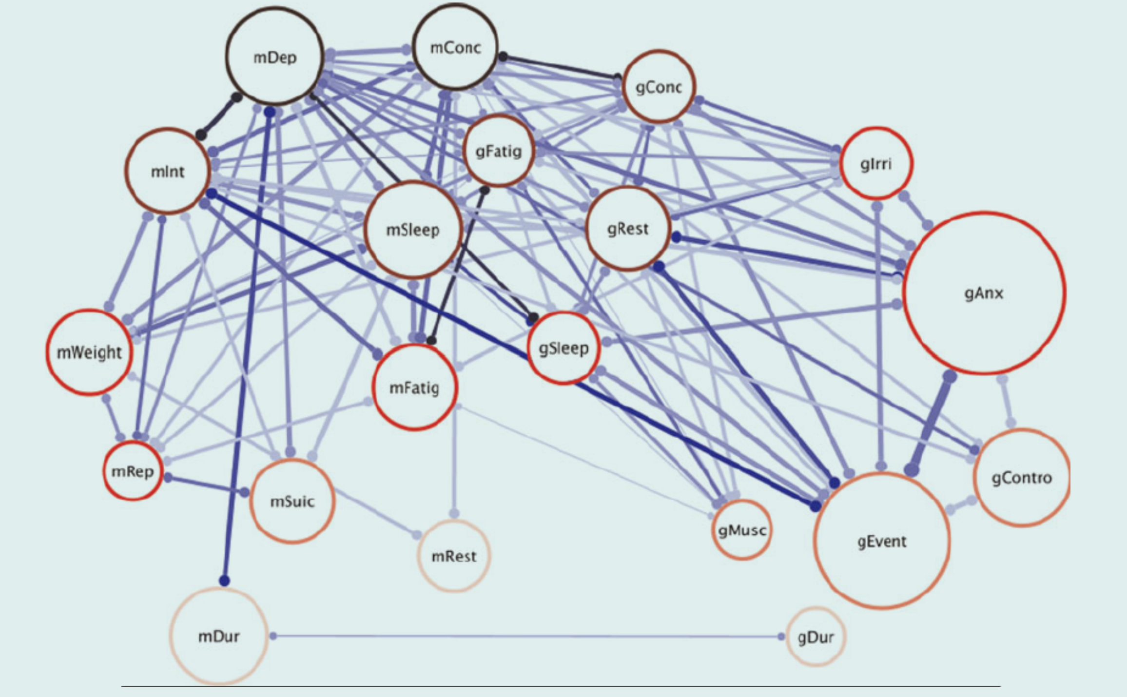
Third, duration (mDur and gDur) is hardly associated with any of the other MDD and GAD symptoms (i.e., few edges are incident in those nodes). This may appear surprising since, in clinical practice, duration is key in determining the presence or absence of a mental disorder. However, if we consider medical illnesses as an analogy, the finding is potentially less surprising: Cancer will be diagnosed if a malignant tumor is present, and that diagnosis is independent of how long the tumor has been present. Thus, we could argue that, in a network approach, MDD is present whenever some symptoms are present without considering the duration of those symptoms. This is not to say that duration is not an important factor at all. Consider again medical illnesses where duration is important in determining the course of action and, subsequently, the probability of full recovery: The longer a malignant tumor has had time to grow and possibly spread, the more difficult it will be to treat it. Duration could fulfill the same role in determining the best course of action for treating mental disorders [Humphry & McGrane, 2010].
For those nodes that seem less significant in networks, are they really insignificant?
Duration of Symptoms
◆ Are there alternative methods for modeling cross-sectional, psychological networks?
A critique of the glasso regularization is that the method was optimized in fields outside of psychology with very different needs, such as high-dimensional data where the number of variables exceeds the number of observations. Which, in psychology, that is not the case. Given our discussion about psychology networks, one may wonder, are there alternative methods for modeling cross-sectional psychological networks?
Here in this article, On Nonregularized Estimation of Psychological Networks, Williams et al. suggested non-regularized alternatives that reduce the false-positive rate and capture the sparsity of psychological networks. This non-regularized alternative set the standard on neighborhood selection, estimating each node’s connections via regression on all other nodes, with justification from AIC and BIC as the decision rule.
The author also suggested using the nonparametric bootstrap approach to estimate the precision matrix directly. But the main takeaway is: there are ways to model cross-sectional psychological networks, and for those non-regularized approaches, they seem to outperform the commonly used glasso regularization at sparsity levels, making these a good choice for low-dimensional psychological networks.
[Check the original article for a detailed view of the study.]
A quick overview of those networks outside of psychology/ psychometrics
We won’t go through this in great detail, but there are a number of areas that may be of interest to you:
fMRI-based Brain Networks: the default mode network, salient network, and frontoparietal network, which link brain regions together with functionality.
Structural Brain Networks: Based on white matter connectivity (DTI)
Connectome: a comprehensive map of neural connections in the brain.
And many more…
Eventually, regardless of the level of analysis, the core principle remains: know what you’re doing, and why you’re doing it. Be deliberate in your methodological choices – understand why you’ve chosen one approach over another, and what trade-offs that entails. Since clear boundaries are hardly elusive, it becomes even more important to define our own theoretical assumptions, remain aware of our own bias and model limitations, continually check whether it aligns with reality… with all those efforts, we’d be fine?