Many things in the real world are gradients/spectrums, but for one reason or another we must put these things into groups and labels. Within the context of networks, communities helps us do just that; they are subgroups of nodes that have high within community connectivity than expected by random chance, given the context of the network. Community detection is a method that allows us to detect different subgroups within a network. This tool helps us identify similarities within a network, and visualize those similarities within groups and differences across groups.
We have to know about the community existing in the first place, and then we need to come up with mathematical definitions that are rigorous enough to classify the different communities.
Formally, community detection is the process of discovering groups in a network where a nodes’ group membership are not explicitly given. It is the process of dividing a network into communities, where each community is some subset of nodes which connect more within their own community than they do outside of their community.
Your definition [what you would tell your grandma]
I am going to use a somewhat strange analogy to explain this, but I promise that this will hopefully make sense. You know those tins that have those really delicious shortbread cookies, but when you open them, they actually have sewing supplies? You have different sewing items like thimbles, needles, strings, safety pins, etc… Some of those items are more related to each other than other items. In this case, the tin of sewing supplies is the network, and different subgroups would be things like items that pierce (pins, needles), items that bind (string, yarn), items that protect you from injury, (thimble), so on and so forth.
Community detection in this case would be us using the associations of the different items in this cookie tin to help us make communities of different objects that have certain characteristics in common. We are trying to find groups of things that are more similar to each other than they are to members of other groups.
Non-exhaustive examples of communities include:
Countries
Species of Animals
Psychological Disorders [symptoms]
The brain
Goals of Community Detection
So now we know what community detection is, but what is our goal with community detection? We are essentially trying to teach a computer/program how to find groups in our data, and from that we can discover some underlying pattern that would not have been visible to us otherwise. To accomplish this, there are certain mathematical expressions we can use that will separate our data into groups. We use an objective function to determine which nodes belong to which groups. In this function, we are essentially asking “are the connections within a group more frequent than the connections outside of a group?”
To put it in simpler terms, we want to find groups, clusters, communities, etc. that share more in common with each other than they do with members of another group. We can use R to help us with this task. For community detection methods, today we will be using the \(\texttt{igraph}\), \(\texttt{stats}\), \(\texttt{mclust}\), and \(\texttt{ppclust}\) libraries.
There are several ways that we could go about this.
Approaches
1. K-Means Clustering
The first approach we have is k-means clustering. This is an unsupervised machine learning model that generates non-overlapping communities from our data. K-means clustering is one of the algorithms we will use to carry out community detection. The way that this algorithm works is that it makes partitions such that the squared euclidean distance between row vectors for any object and the centroid vector of its respective cluster is at least as small as the distances to the centroids of the remaining clusters. With this algorithm, a node can only belong to one community.
The centroid is the mean position of all points in the cluster.
To give a simpler breakdown of how this algorithm works:
We specify our \(k\) (number of groups) and randomly assign \(n\) (our subjects) to one of \(k\) clusters
Calculate the means for each \(k\)
Shuffle subjects to clusters where their distance is minimized
Recalculate means and repeat to convergence
In this case, our convergence criteria is the within-cluster sums of squares. WCSS is a method used to determine the optimal number of clusters to include. This is incredibly helpful evaluating the compactness of our clusters. We are measuring the sum of squared distances between each data point and the centroid of its assigned cluster. Points across different subgroups have no influence on their calculation of a different subgroup.
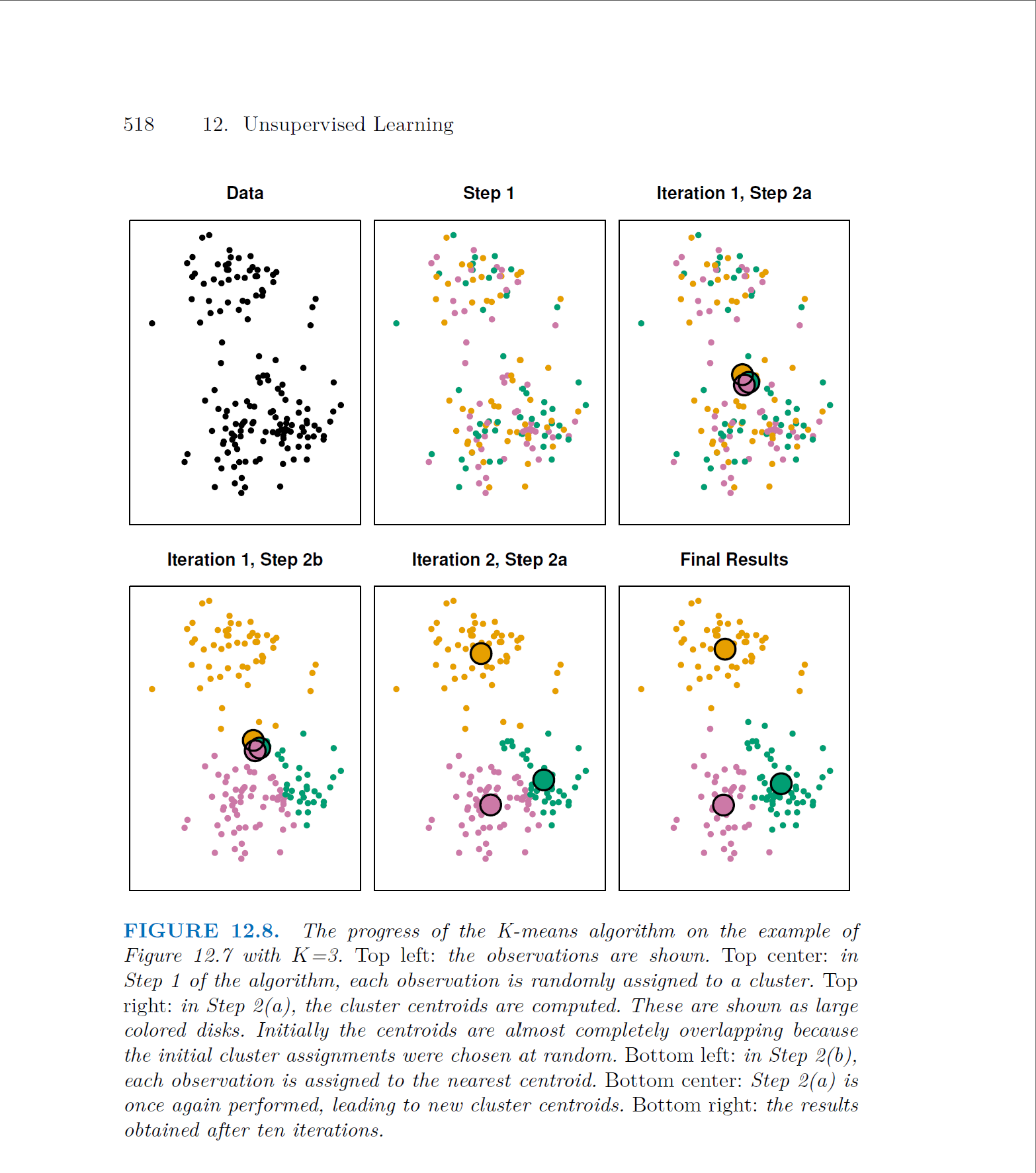
This page is from Introduction to Statistical Learning - Second Edition. Here we can see k-means clustering in action. We see the data go from an unclassified state, to partitioning into different clusters, to finally having that within cluster sums of squares minimized in the final results panel.
Here is what each part of the function is telling us:
\[ \sum_{j=1}^{C} \sum_{i=1}^{n_j}\] are the total number of communities to partition, and
\[ ||x_{i} - \bar{x}_{j}||^{2} \] is the euclidean distance between individual i’s values on a vector of variables x, and the jth community means \(\bar{x}_{j}\).
The goal of this objective function is that we are trying to minimize the within-cluster sum of squares.
Now that we have a theoretical understanding of k-means clustering and what is going on, let’s use R to implement community detection.
Here, we are reading in our code and initializing the data we will be using, the number of groups that we want to find, and the number of nodes that we want in each group. We also load in the packages we will need to analyze this data.
library(igraph)
Attaching package: 'igraph'
The following objects are masked from 'package:stats':

    decompose, spectrum
The following object is masked from 'package:base':

    union
library(stats)library(mclust)
Package 'mclust' version 6.1.1
Type 'citation("mclust")' for citing this R package in publications.
Next, will create a variable called results.1 and in that variable, we use lapply on our data to apply our k means cluster algorithm. We are going to create up to 11 different clusters. The next part of lapply is us telling R what function we want to run on our data. In the kmeans function, we are passing
the adjacency matrix (adjacency.matrix)
centers: how many communities we think that there are
iter.max: how many times we want to kmeans algorithm to shuffle our data?
nstart: how many times should we randomly put people into groups??
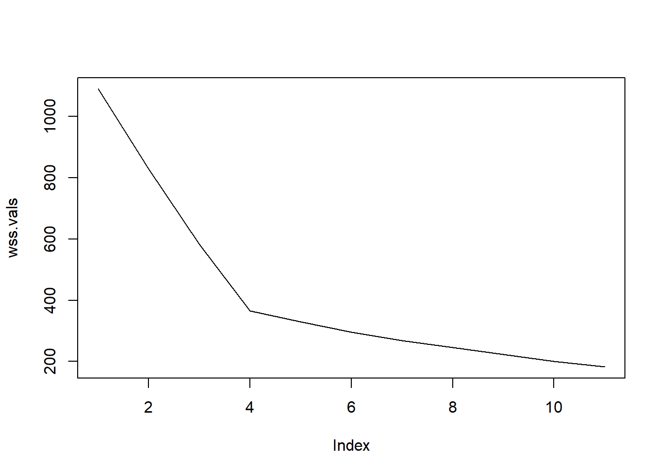
After running our code, we now need a way to visualize how the within-cluster sum of squares changes as the number of communities increase. We can use a scree plot to visualize this.
Question: What does the general trend of this graph indicate to us?
As the number of communities increase, the within cluster sum of squares deceases.
In that case, we should probably partition our data to where we have a large number of groups, preferably to match how many points of data we have in our dataset.
Question: Why might that be a problem for us?
If we increase the number of groups to be a really large number, then each point will just be its own group!
We would essentially be back at square one. In the case where our number of groups is equal to the number of data entries, each point would be its own group. Going back to our objective function, if we take an observation and subtract it by the mean (which would also be itself), then our error would be zero!
So generally, we can deduce that adding more communities lowers the WCSS. However, we want a way to find the “optimal” number of communities we should have in our k-means cluster algorithm. To do this, we use the elbow trick to find the optimal number of communities. We find the inflection point in the graph where the line gives us a drastic decease in the error, but not so much in the following values
Question: which point in this graph is the elbow?
The elbow is located where the number of groups is equal to 4.
It appears that at four groups, we see a drastic decrease in the within cluster sum of squares. The subsequent values following 4 do not seem to offer that much of an improvement.
2. Fuzzy C-Means Clustering
Having a tool like K-means clustering is incredibly helpful for creating hard boundaries for groups in our data. However, we may want other methods of representing what groups our data belongs to.
Fuzzy c-means clustering is a very similar algorithm to k-means clustering. We are still estimating the likelihood of membership across different groups, however, a key difference is that nodes can belong to multiple groups (hence the name “fuzzy” means clustering).
To give an example of how this would work, fuzzy clustering would indicate the likelihood of classifying if an individual belongs to group A, and a separate likelihood that they belong to group B (or however many different groups that you have).
Can you think about why we might want this “fuzziness”. When and where might this be useful to us?
There are two very important differences between this and the objective function for K-means clustering.
\(\sum_{i=1}^{N}\) is the sum from the first individual to the \(N{th}\) individual. This is different because rather than calculating the error of a specific group, we are calculating the difference from every person and every group.
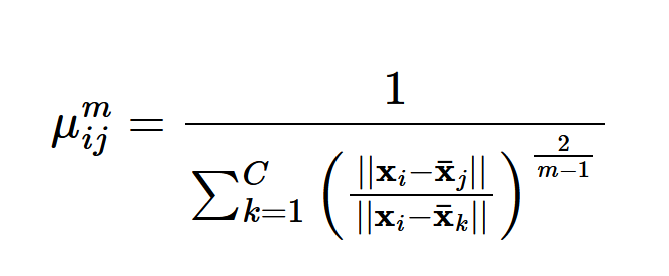
\(\mu_{ij}^{m}\) is known as the fuzzifier. This is the membership degree between the \(i^{th}\) and \(j^{th}\) community based on the fuzzifier, \(m\). This is the term that greatly changes the function. Let’s go deeper into it!
The Fuzzifier
Here is our equation for the fuzzifier:
It is quite an intimidating equation, but lets break down the components:
\(\mu_{ij}^{m}\) is known as the membership degree for each subject \(i\) into group \(j\) given \(m\). It is a fraction that depends on the ratio of the distance between subject \(i\) and group \(j\) compared to the distance of subject \(i\) and clusters 1 to \(C\)-not including \(j\). Finally, we exponentiate this beauty to the \(2/(m-1)\) power.
This equation accomplishes some interesting things:
As a result, all individuals will belong to every cluster, but they will have varying degrees of membership within said clusters
High degree individuals are more confidently within a specific cluster
Low degree individuals in all group may be fuzzy in their membership
\(m\) also has some interesting properties. When \(m\) is exactly 1, we have a case where it exhibits properties similar to k-means
As \(m\) approaches infinity, what happens to our boundaries?
As \(m\) approaches infinity, the boundaries for our clusters will become incredibly blurry. This means that all clusters receive almost equal membership, regardless of distance.
Fuzzy clustering draws from fuzzy logic and allows for cluster membership to be determined based on degree weights instead of yes/no classification. As our fuzzifier approaches 1, we have a hard clustering solution. As our fuzzifier approaches infinity, we have almost no boundaries between our data.
To put a bow on the fuzzifier, its role is to weight the influence of subject \(i\) to each \(j\) groups. If a subject does not belong to a community, it will still affect the calculation of its centroid and contribute to the within cluster error. The thing to note is that it will be weighted drastically less than the individuals who are confidently in that community.
Given the two different algorithms, we can draw upon some similarities and differences between them. Both algorithms attempts to partition data into clusters with the difference being k-means is non-overlapping while fuzzy c-means does have some overlap between the data. Both algorithms help us classify our network/data into communities.
What other similarities/differences do you notice between the two?
Without further adieu, let’s use R to implement this!
We can choose to view as many groups as we want, however, we may find that we have extracted too many groups from our data.
(BONUS) - Walktrap
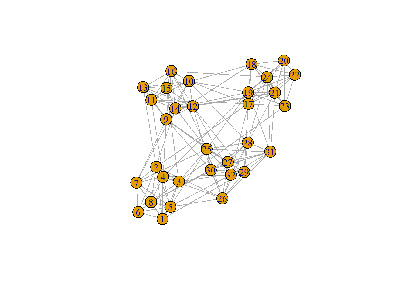
The last algorithm that we will talk about today is the walktrap. Let’s say that we have a graph such as the one below:
ng =graph_from_adjacency_matrix(adjacency.matrix, mode ="undirected", diag =FALSE,weighted =TRUE)plot(ng)
We are placed on node 1. From node one, we take a proverbial walk through the network. From this, we can ask the following question:
“What is the probability that you will go from node 1 to any other node in a walk of length \(s\)?”
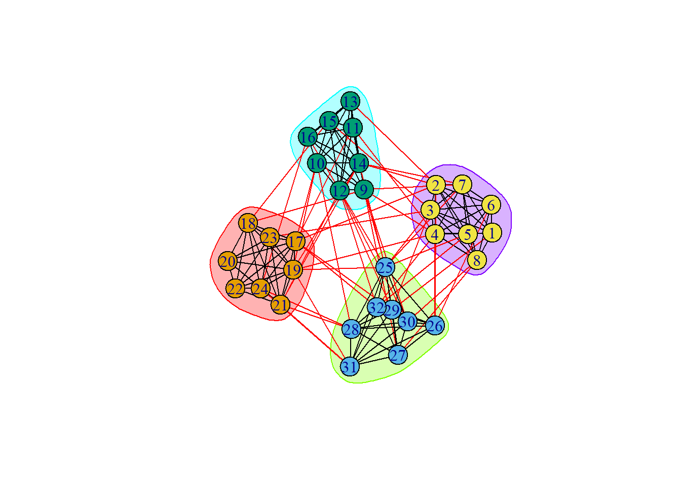
If we do this process many times, we will find that our walks will be confined to certain communities. This is the informal idea behind walktrap. Here is the end result of that process:
groups =cluster_walktrap(ng)plot(groups, ng)
I am not going to even attempt to pretend to know the math behind how walktrap work as I do not want to mislead the reader. However I highly recommend that you look Pascal Pons and Matthieu Latapy’s 2006 paper titled “Computing Communities in Large Networks Using Random Walk” as it is very interesting and explains the process in great detail.
Finally, we want a way to see how well our models performed with detecting communities. Most of the time, we do not know what the true group memberships are. However, we are able to assess the accuracy in this scenario since we do have the true group memberships.
The adjusted rand index (or ARI for short) is a validation metric between 0 and 1 that is meant to quantitatively evaluate and compare our clustering results. The “adjusted” part of the name comes from the fact that compared to the rand index, ARI is accounting for baseline similarity that can pop up randomly.
Above we have the model performance of k-means, c-fuzzy means, and walktrap laid out for us. I think that you will be pleased to discover that an ARI of 1 means that we have perfect performance across all three models! An ARI of 0.90 and up indicates that our models are doing a fantastic job of classifying our data.
I hope you walked away from this article learning more about community detection and the various methods we can use to apply it!