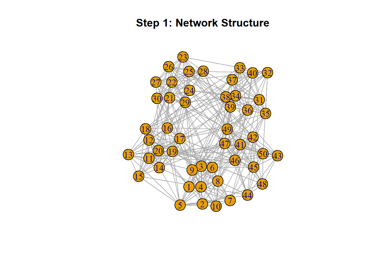
We’ve already talked some about communities in this class, specifically when it came to finding measures of centrality. Today, we will be covering some methods for actually finding subgroups, or communities, within the network. As I have been working on social network analyses, I will be integrating examples, when applicable, from rhesus macaques from the California National Primate Center (CNPRC), in today’s talk.
The objective of K-means clustering is to partition data (in this case, nodes and their links) into K clusters or classes. With jargon, the K-means method constructs the partitions (or splits) so that the squared Euclidean distance between the object (node) and the centroid of its cluster is as 1) as small as possible and 2) as small as the distance from the centroids of remaining clusters (Steinley (2006)).
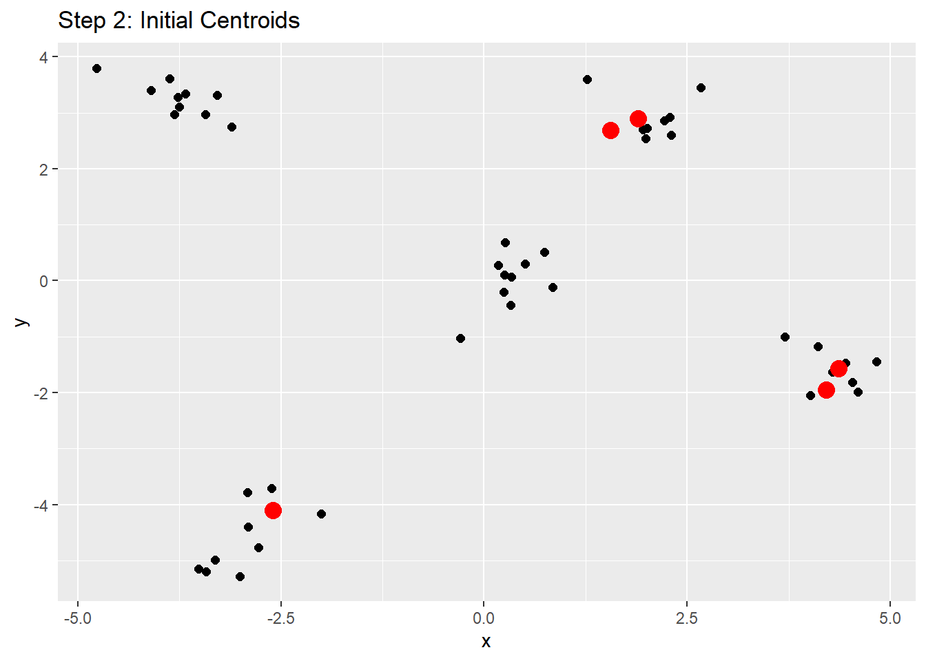
The centroid is the average point of a cluster found by averaging the values of each variable over all objects in the cluster. According to the literature, the true computational method for finding the initial centroids in a K-means cluster analysis consists of:
  1. defining "initial seeds" defined by a vector from the data
  2. the squared Euclidean distance between the seeds and objects are found
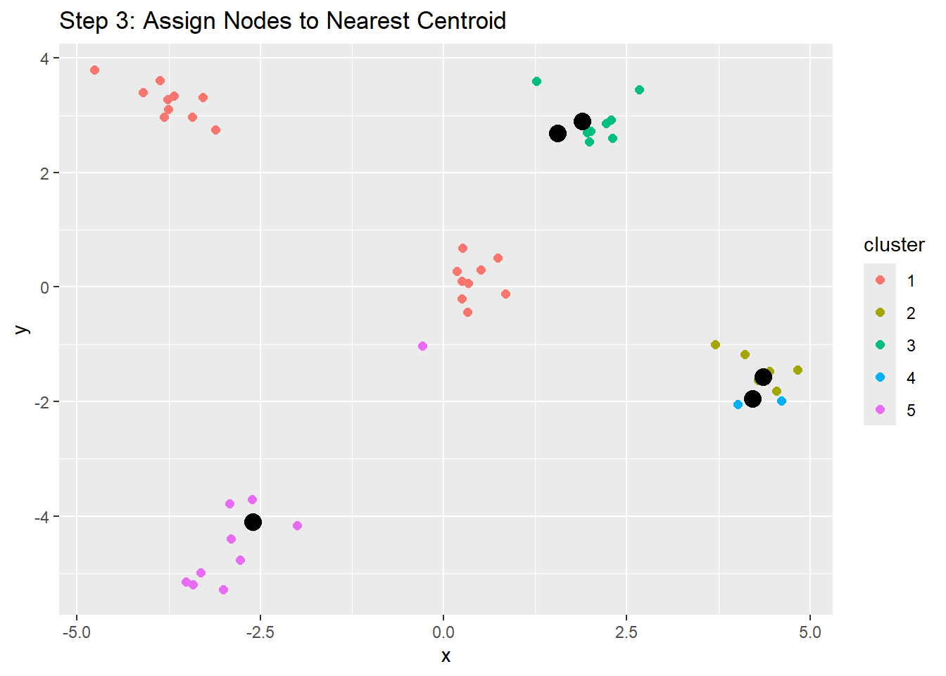
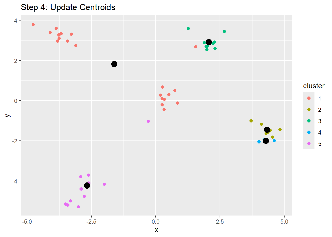
K-means clustering then iterates over the initial seeds, or centroids, until the least distance between the centroids and objects can be found, resulting in multiple clusters with centroids and objects around it. The approach is:
  1. In iterates over the distances, moving the centroids around objects so that the least distance is found
  2. These new cnetroids are calculated, thereby updating "cluster membership"
  3. Once no objects can be moved between clusters, the K-means clusters have been found. Yay!
Therefore, Steinley (2006) writes that that objective function of K-means clustering is to minimize the error sum of squares (SSE), as in the equation below:
\[ SSE = \sum_{j=1}^{P} \sum_{i \in C_k} \sum_{k=1}^{K} (x_{ij} - \bar{x}^k_{j})^2 \]
\(K\) = number of clusters
\(C_k\) = set of objects (nodes) in cluster \(k\)
\(x_{ij}\) = value of the \(j\)-th variable for the \(i\)-th object
\(\bar{x}_{kj}\) = mean of the \(j\)-th variable for cluster \(k\) (centroid)
The inner term, \((x_{ij} - \bar{x}^k_{j})^2\), is the most important part. This is the squared distance between a node and the centroid. If the node is close to the centroid, the result is a small value.
We sum over variables, \(\sum_{j=1}^{P}\), to get the total distance for a given node. We then add up the distances for all nodes within a cluster,\(\sum_{i \in C_k}\), and then sum across all clusters, \(\sum_{k=1}^{K}\), to get the total error for the entire clustering solution.
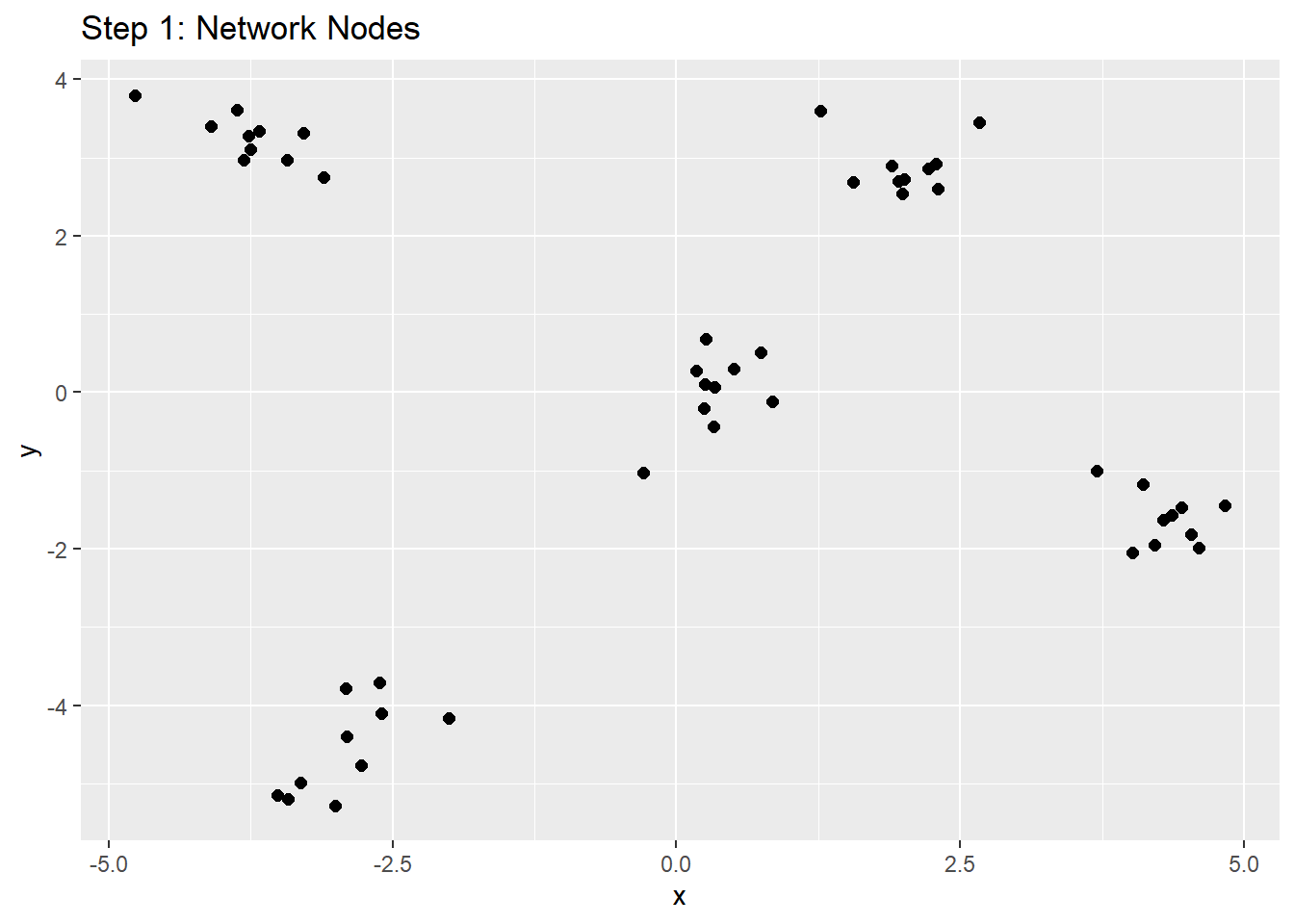
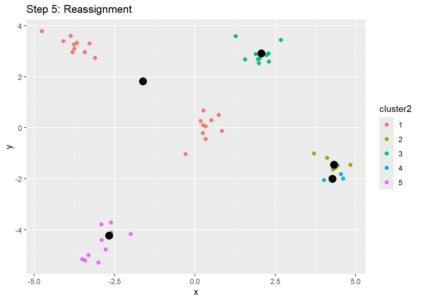
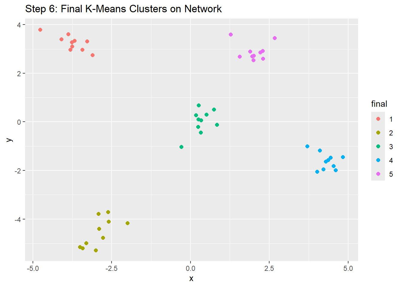
While this took us step by step in how k-means clusters are created, let’s approach this more intuitively. So essentially, we are assigning K groups and putting people into groups. We want to minimize the distance from group mean to each individual node, thereby putting everyone into the group/cluster that is most similar to them. Let’s think of centroids as descriptors in order to make it more comprehensible - these are just average descriptors and the groups are clustering around that average descriptor.
An important note is deciding on how many clusters to have. We can’t be too exact - if there is a centroid per individual node, the k-means would be too exact, the centroid would become the node, and there would be no actual groupings.
To visualize this, let’s look at this example from Jonathan. Say we have x amount of nodes and are trying to find a clustering solution between 1 and 17 groups. We put this through some cool code and find the within groups sum of squares for each cluster solution, with the goal of looking for the point at which adding more clusters stops meaningfully reducing WSS. It spits out the following figure:
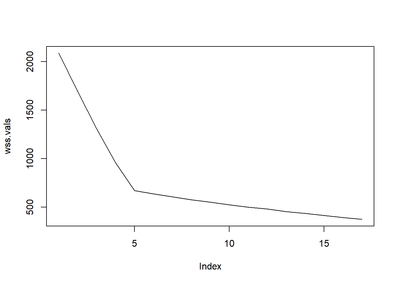
An elbow is at around 5! Here, we are looking for where the Within Group Sum of Squares is minimized, but at 5 we start to see an elbow and very slow leveling off. The improvement after the elbow, so after 5 groups, is very minimal and the subsets of groups start to become very small and more specific, eventually coming to a point where nodes start to become their own groups. This indicates high levels of error and an over-fitting of clustering. The ratio, with regards to WSS, before and after the elbow serves as a good indicator of where to cut off the number of clusters that are ideal.
As a final note, it is important to note that k-means clustering is based on connection patterns from the adjacency matrix rather than directly detecting communities in the graph structure. The reason to keep this in mind, is that k-means clustering is grouping nodes with similar connection profiles in a space rather than dense connections. A helpful reminder is to think of the centroids as abstract descriptors, as said above. Therefore, the clusters can be thought of as groupings of similarly-behaving nodes.
We left off with this question of how to decide the amount of clusters that are appropriate for organizing the nodes. Where are there cutoffs in creating groups? How are groups partitioned? To answer these questions, we turn to Fuzzy c-Means Clustering!
K-means clustering partitions nodes into discrete clusters and groups all nodes. A key limitation is that it forces groups, hard assigning nodes when there is a possibility that the nodes should not be grouped into a particular cluster. In real systems, this assumption can be too strict. In fuzzy c-means clustering, we can see the partial membership across multiple clusters and get the “probability” that nodes belong in certain clusters.
Fuzzy c-means introduces a membership weight which represents the degree to which a node, say \(i\), belongs to cluster \(k\). The function described in Park, Chow, and Molenaar (2024) is:
\[ J(U,X) = \sum_{j=1}^{C} \sum_{i=1}^{N} u_{ij}^m \| x_i - \bar{x_j} \|^2 \]
The terms are:
\(u_{ij}^m\) = element in the larger \(U\) membership degree matrix. This is bounded between 0 and 1. For any individual, the sum of their membership across all communities must equal 1.
\(U\) = membership matrix (rows sum to 1 for each node)
\(N\) = total number of nodes
\(C\) = total number of communities for a given \(m\) (\(m\) > 1)
\(\bar{x_j}\) = centroid of cluster \(j\)
\(m\) = the fuzzifier, determines the fuzziness of the community assignment
As \(m\) -> 1, the membership values become binary and the model approaches the k-means clustering. (We’ll talk about this later!)
The inner term, \(|x_i - \bar{x_j} \|^2\), just as in k-means clustering, represents the squared distance between a node and a cluster centroid. The fuzzy c-means cluster weights this distance by the membership value, \(u_{ij}^m\). If a node strongly belongs to a cluster, the weight will be higher.
For every node \(i\) and every cluster \(j\), we compute the distance to the centroid, weight that distance by how strongly the node belongs to the cluster, and then sum everything across all nodes (\(\sum_{i=1}^{N}\)) and clusters (\(\sum_{j=1}^{C}\)).
Like k-means clustering, the function aims to find the partitions that result in the smallest possible distance between data points and their centroids, however, in c-means, we are finding the smallest possible total total weighted distance. The degree of membership is inversely related to the distance between the data point and its assigned centroid. Therefore, the closer a point is to the centroid relative to other centroids, the higher its membership degree for that cluster.
The major difference between the two, as we’ve touched on, is that k-means clustering has the centroid be an average of the nodes around it, within the cluster. This results in discrete, forced groupings in which all nodes are placed within a group. However, the confidence of a node actually belonging to that cluster may not be high. In fuzzy c-means, the weighted centroids results in assigning membership weights across all clusters. These “probabilities” or “confidence thresholds”, to put it simply, allows for nodes to exist outside of clusters and for clusters to be more precise and accurate.
Fuzzy c-means produces a membership matrix, where each node has weights (probabilities) of belonging to each cluster. It also allows for changing the amount of groups, so that you can “play” with finding the best split of groupings. As stated, these benefits of the fuzzy c-means allows the identifying of core members in a given cluster (higher weight for one cluster), identifying uncertainty in clustering, and in identifying “fringe” nodes.
 1  2  3  4  5  6  7  8  9 10 11 12 13 14 15 16 17 18 19 20 21 22 23 24 25 26
 2  2  2  2  2  2  2  2  2  2  3  3  3  3  3  3  3  3  3  3  5  5  5  5  5  5
27 28 29 30 31 32 33 34 35 36 37 38 39 40 41 42 43 44 45 46 47 48 49 50
 5  5  5  5  4  4  4  4  4  4  4  4  4  4  1  1  1  1  1  1  1  1  1  1
Cluster 1 Cluster 2 Cluster 3 Cluster 4
1 0.58 0.13 0.15 0.14
2 0.54 0.15 0.16 0.15
3 0.53 0.16 0.16 0.15
4 0.53 0.16 0.16 0.16
5 0.54 0.15 0.15 0.17
6 0.53 0.15 0.17 0.16
7 0.59 0.13 0.15 0.13
8 0.58 0.13 0.15 0.14
9 0.49 0.16 0.18 0.17
10 0.50 0.16 0.17 0.16
11 0.14 0.13 0.12 0.62
12 0.14 0.13 0.11 0.62
13 0.14 0.12 0.11 0.64
14 0.16 0.14 0.14 0.56
15 0.12 0.10 0.09 0.69
16 0.15 0.13 0.14 0.58
17 0.15 0.14 0.14 0.56
18 0.15 0.13 0.13 0.59
19 0.14 0.13 0.12 0.60
20 0.16 0.15 0.15 0.54
21 0.14 0.60 0.12 0.14
22 0.16 0.54 0.15 0.15
23 0.14 0.60 0.13 0.13
24 0.14 0.59 0.13 0.14
25 0.14 0.59 0.14 0.13
26 0.14 0.60 0.13 0.13
27 0.14 0.61 0.12 0.13
28 0.13 0.63 0.12 0.11
29 0.15 0.58 0.13 0.14
30 0.17 0.52 0.15 0.16
31 0.15 0.12 0.61 0.12
32 0.13 0.12 0.63 0.12
33 0.15 0.14 0.58 0.13
34 0.17 0.16 0.52 0.15
35 0.13 0.10 0.66 0.10
36 0.14 0.11 0.64 0.11
37 0.16 0.14 0.56 0.14
38 0.16 0.13 0.59 0.13
39 0.15 0.13 0.60 0.12
40 0.14 0.13 0.61 0.12
41 0.31 0.22 0.24 0.23
42 0.31 0.25 0.22 0.21
43 0.29 0.24 0.24 0.23
44 0.33 0.22 0.22 0.23
45 0.30 0.22 0.24 0.24
46 0.28 0.23 0.24 0.25
47 0.30 0.23 0.24 0.22
48 0.32 0.23 0.22 0.23
49 0.27 0.27 0.23 0.23
50 0.30 0.23 0.24 0.23 Cluster 1 Cluster 2 Cluster 3 Cluster 4 Cluster 5
1 0.12 0.60 0.10 0.10 0.08
2 0.13 0.57 0.10 0.10 0.10
3 0.14 0.54 0.11 0.11 0.11
4 0.14 0.53 0.11 0.11 0.11
5 0.13 0.56 0.11 0.10 0.10
6 0.15 0.51 0.11 0.12 0.11
7 0.13 0.60 0.09 0.10 0.09
8 0.12 0.60 0.09 0.10 0.09
9 0.15 0.49 0.12 0.13 0.12
10 0.14 0.51 0.11 0.12 0.11
11 0.12 0.09 0.61 0.09 0.09
12 0.11 0.10 0.60 0.09 0.10
13 0.10 0.10 0.64 0.08 0.08
14 0.13 0.12 0.54 0.11 0.11
15 0.10 0.08 0.67 0.07 0.08
16 0.12 0.11 0.57 0.10 0.10
17 0.14 0.11 0.54 0.11 0.11
18 0.12 0.11 0.58 0.10 0.10
19 0.12 0.10 0.59 0.09 0.10
20 0.14 0.12 0.52 0.11 0.12
21 0.12 0.10 0.11 0.09 0.57
22 0.13 0.12 0.11 0.11 0.53
23 0.13 0.10 0.10 0.10 0.56
24 0.12 0.10 0.10 0.10 0.58
25 0.12 0.10 0.10 0.10 0.59
26 0.11 0.10 0.09 0.09 0.61
27 0.11 0.10 0.09 0.09 0.61
28 0.13 0.10 0.09 0.10 0.60
29 0.13 0.11 0.11 0.10 0.55
30 0.14 0.13 0.12 0.11 0.50
31 0.12 0.11 0.09 0.60 0.09
32 0.10 0.09 0.08 0.64 0.09
33 0.12 0.11 0.10 0.56 0.10
34 0.14 0.13 0.12 0.49 0.12
35 0.11 0.10 0.08 0.62 0.08
36 0.11 0.10 0.08 0.62 0.08
37 0.12 0.11 0.11 0.56 0.10
38 0.12 0.12 0.10 0.58 0.09
39 0.11 0.11 0.09 0.59 0.09
40 0.11 0.10 0.09 0.61 0.09
41 0.53 0.13 0.12 0.12 0.11
42 0.62 0.11 0.08 0.09 0.10
43 0.57 0.11 0.10 0.11 0.11
44 0.57 0.13 0.10 0.10 0.10
45 0.50 0.14 0.13 0.13 0.11
46 0.52 0.12 0.12 0.12 0.11
47 0.53 0.13 0.11 0.12 0.11
48 0.60 0.11 0.10 0.09 0.09
49 0.48 0.13 0.12 0.12 0.14
50 0.58 0.11 0.10 0.10 0.10 Cluster 1 Cluster 2 Cluster 3 Cluster 4 Cluster 5 Cluster 6
1 0.08 0.10 0.07 0.08 0.15 0.51
2 0.08 0.11 0.08 0.09 0.16 0.48
3 0.09 0.12 0.09 0.09 0.16 0.45
4 0.09 0.12 0.09 0.09 0.17 0.44
5 0.10 0.11 0.08 0.08 0.16 0.47
6 0.09 0.12 0.09 0.10 0.18 0.42
7 0.08 0.11 0.07 0.08 0.16 0.50
8 0.08 0.11 0.07 0.08 0.16 0.51
9 0.10 0.13 0.10 0.10 0.18 0.40
10 0.09 0.12 0.09 0.10 0.16 0.43
11 0.53 0.10 0.08 0.07 0.13 0.08
12 0.52 0.10 0.08 0.07 0.14 0.09
13 0.56 0.09 0.07 0.07 0.13 0.08
14 0.46 0.11 0.09 0.09 0.15 0.10
15 0.59 0.09 0.07 0.06 0.13 0.07
16 0.49 0.10 0.08 0.09 0.14 0.09
17 0.46 0.12 0.09 0.09 0.15 0.10
18 0.49 0.10 0.08 0.09 0.15 0.09
19 0.50 0.10 0.08 0.08 0.14 0.09
20 0.44 0.12 0.10 0.09 0.15 0.10
21 0.09 0.11 0.49 0.08 0.15 0.09
22 0.10 0.11 0.45 0.09 0.15 0.10
23 0.09 0.12 0.47 0.08 0.16 0.09
24 0.09 0.11 0.50 0.08 0.14 0.08
25 0.08 0.10 0.51 0.08 0.13 0.08
26 0.08 0.09 0.54 0.08 0.13 0.08
27 0.08 0.10 0.54 0.07 0.13 0.08
28 0.08 0.11 0.50 0.08 0.15 0.08
29 0.09 0.11 0.46 0.09 0.16 0.09
30 0.10 0.12 0.42 0.10 0.15 0.11
31 0.07 0.10 0.08 0.51 0.14 0.09
32 0.07 0.09 0.07 0.56 0.12 0.08
33 0.09 0.11 0.09 0.48 0.14 0.09
34 0.10 0.12 0.10 0.41 0.16 0.11
35 0.07 0.10 0.07 0.53 0.15 0.09
36 0.07 0.10 0.07 0.54 0.14 0.09
37 0.09 0.11 0.09 0.48 0.14 0.10
38 0.08 0.10 0.08 0.50 0.14 0.10
39 0.08 0.10 0.08 0.51 0.14 0.09
40 0.08 0.10 0.08 0.53 0.13 0.08
41 0.09 0.40 0.08 0.09 0.23 0.10
42 0.07 0.49 0.08 0.07 0.21 0.08
43 0.09 0.45 0.09 0.09 0.20 0.09
44 0.08 0.44 0.08 0.08 0.22 0.10
45 0.10 0.38 0.09 0.10 0.22 0.11
46 0.10 0.40 0.09 0.09 0.22 0.10
47 0.08 0.41 0.09 0.09 0.23 0.10
48 0.08 0.46 0.07 0.07 0.22 0.09
49 0.09 0.37 0.11 0.10 0.23 0.10
50 0.08 0.45 0.08 0.08 0.21 0.09
This example, taken from a lecture given by Jonathan, shows an example of fuzzy c-means clustering. To make a long story short, a fuzzy c-means clustering resulted in two distinct clusters (red and cyan) and a fringe grouping in black that is not a true third cluster. Instead, these data points are those that do not belong in either of the other two clusters but also don’t cluster together. In his example, he hypothesized that these were individuals exhibiting symptoms of Major Depressive Disorder but also getting treatment/care for this diagnosis. This serves as a good example of how the fuzzy c-means can result in more precise clusters.
Gaussian Mixture Models provide a probabilistic framework for clustering, where each cluster is modeled as a Gaussian distribution. Under specific conditions, GMMs have identical results as k-means clustering. According to Park, Chow, and Molenaar (2024) and Steinley (2006), when the model uses an identity covariance matrix, the k-means clustering results become the same as those from a Gaussian Mixture Model. When there are hard assignments, spherical covariances, and equal variance, the K-means becomes the GMM.
Fuzz c-means “softens” and extends k-mean clustering, by accounting for weighted memberships and “fuzziness”. However, when the \(m\), or membership weights, approach 1, the fuzzy c-means converges to k-means. The memberships are forced to be binary, and therefore it becomes the hard, forced clustering present in k-means (Park, Chow, and Molenaar (2024)).
As with K-means clustering, the user is the one who determines the number of clusters, based on theory, previous knowledge, or an informed hypothesis (Park, Chow, and Molenaar (2024)). These clusters then need to be questioned.
How do we know whether the clusters we get are legitimate?
Jonathan points out an example using ionic and polar covalent bonds - while it is often taught that there are differences in the bonds and their behaviors, the cutoffs in electronegativity to organize those bonds are not agreed upon. In just one textbook, different cutoffs, or clusters where each bond should be differentiated, differ. Does this mean that the clusters don’t really exist? Are we not precise enough in our partioning? Should a third group exist or are there just exceptions?
To answer these questions, we need to analyze the assumptions behind the community detection tests and examine how accurate and precise our tools for detection are.

Modularity is commonly used for detecting communities. Modularity is defined directly from the graph structure instead of a geometric feature space like k-means clustering and fuzzy c-means. Modularity is its own concept wherein the heuristic is comparing the number of connections within the community to the expected number of connections you would obverse by chance. With this thinking, one node should be more connected to members of their community than to anyone else, based on random chance (Brusco, Steinley, and Watts (2024b); Brusco, Steinley, and Watts (2024a); Gates et al. (2016)).
Modularity compares the number of observed edges within a community and compares it to the expected number of edges under a random network model (\(\frac{k_ik_j}{2m}\)). Therefore, if nodes within a community have more connections among themselves than expected by chance, then a community structure would be deemed as strong (Fortunato and Barthelemy (2007)).
There are some limitations to this line of thinking. For example, small communities within a network could be potentially folded into other ones, thereby not detected. The size and density of a network greatly influences modularity and it also overlooks how the connections exists by only considering edge counts and not structure. By simply comparing number of connections, it can overlook the same amount of connections made by different partitions, thereby equating communities that might look very different in their connections.
As a result, modulairty can be interpreted as a useful heuristic rather than a definitive measure of community structure. This then begs the question: what other cluster quality metrics are there?
A word from esteemed Dr. Jonathan Park
The question of cluster quality is a natural extension. Are my distinctions/partitions/cuts/splits actually clean, meaningful, and appropriate?
Partition Entropy (PE) is a cluster quality index to evaluate how “clean” or “fuzzy” the clusters from fuzzy c-means clustering are. PE calculates the average fuzzy entropy within the membership degree matrix, thereby assessing the amount of uncertainty involved in assigned the nodes to specific communities (Park, Chow, and Molenaar (2024)).
\[ PE = - \frac{1}{N} \sum_{j=1}^{C} \sum_{i=1}^{N} u^m_{ij} \log(u^m_{ij}) \] where:
The inner term, \(u^m_{ij} \log(u^m_{ij})\), measures the uncertainty of a node’s membership in a given cluster. If a node strongly belongs to one cluster (\(u^m_{ik}\) -> 1), there is low uncertainty. For every node (\(\sum_{i=1}^{N}\)) and every cluster (\(\sum_{j=1}^{C}\)), we calculate how uncertain the membership is, and then average this uncertainty across all nodes.
The PE index ranges from 0 to 1, with values of 0.0 or as close to 0.0, indicating high-quality partitions. A score of 0 is a perfect clustering. Conversely, higher values (towards 1) indicate fuzzier or more ambiguous partitions.
The silhouette index measures how well each node fits within its assigned cluster compared to other clusters. For a given node, the silhouette index compares the average distance to 1) nodes in its own cluster and 2) to the average distance to nodes in the nearest alternative cluster. Values can range from -1, where the node is misclassified in its cluster, to +1, where the node is a perfect fit for its cluster.
The formula is:
\[ s(i) = \frac{b_{ik} - a_{ij}}{\max\{a_{ij},\, b_{ik}\}} \] where
The denominator is a normalization term that selects whichever value is greater: - the average distance between a subject and its assigned neighbors OR - the average distance between a subject and the members of the closest neighboring cluster
The silhouette index provides a measure of cluster separation and cohesion.
The Adjusted Rand Index (ARI) evaluates how similar a clustering solution is to a known or “true” grouping, where:
Since 0 is chance, an ARI of around 0.7 is considered a decent recovery and accepted as a good clustering fit. The ARI is considered a better tool for evaluating the fit of clustering partitions (Brusco, Steinley, and Watts (2024a); Gates et al. (2016)).
\[ ARI = \frac{\binom{N}{2}(a + d) - \left[(a + b)(a + c) + (c + d)(b + d)\right]} {\binom{N}{2}^2 - \left[(a + b)(a + c) + (c + d)(b + d)\right]} \]
where:
In summary, the ARI is designed to compare the number of correct clusters relative to incorrect clusters, correcting for correct decisions by random chance.
While methods like k-means clustering rely on geometrics representations and methods like modularity operate on the graph structure, spectral clustering transforms networks into a space where geometric clustering can be applied (Brusco, Steinley, and Watts (2024a)).
Eigenvector centrality transforms the axis of the geometric space where the nodes lie so that the x-axis becomes the through line of the data, better described as the influential axis or most common descriptor. The y-axis is then the deviation from that x-axis. In spectral clustering, we can think of the axes being similar to the ones transformed by the eigenvector centrality metric, and through this, the dimensions “bend” together in the Euclidean space. The Laplacian is the diagonalized Degree - Adjacency Matrix, in which the network is rewritten in a way that makes connected nodes appear closer together in space (Brusco, Steinley, and Watts (2024a); MacMahon and Garlaschelli (2013)). This has the unique property of normalizing degree differences across nodes.
Instead of looking at the highest eigenvalues, for spectral clustering, we are looking specifically for the fringe cases, so at the lower end of the spectrum. This is where we can start to look at unique differences.
Taking our example of 50 individuals:
 [1] 2 2 2 2 2 2 2 2 2 2 4 4 4 4 4 4 4 4 4 4 5 5 5 5 5 5 5 5 5 5 1 1 1 1 1 1 1 1
[39] 1 1 3 3 3 3 3 3 3 3 3 3
Each number represents the cluster label assigned by k-means on the spectral embedding. The first 10 nodes are a mixture of being clusters 2 and 4, while the remaining nodes fit more cleanly into clusters. We specified 5 true groups with 10 nodes in each and we can see that the spectral clustering did recover some groups, while others were mixed. This can indicate the structure of clusters 2 and 4 are less well separated in the network. Spectral clustering reveals that not all communities are equally well-defined—some emerge clearly, while others overlap in their connectivity patterns.
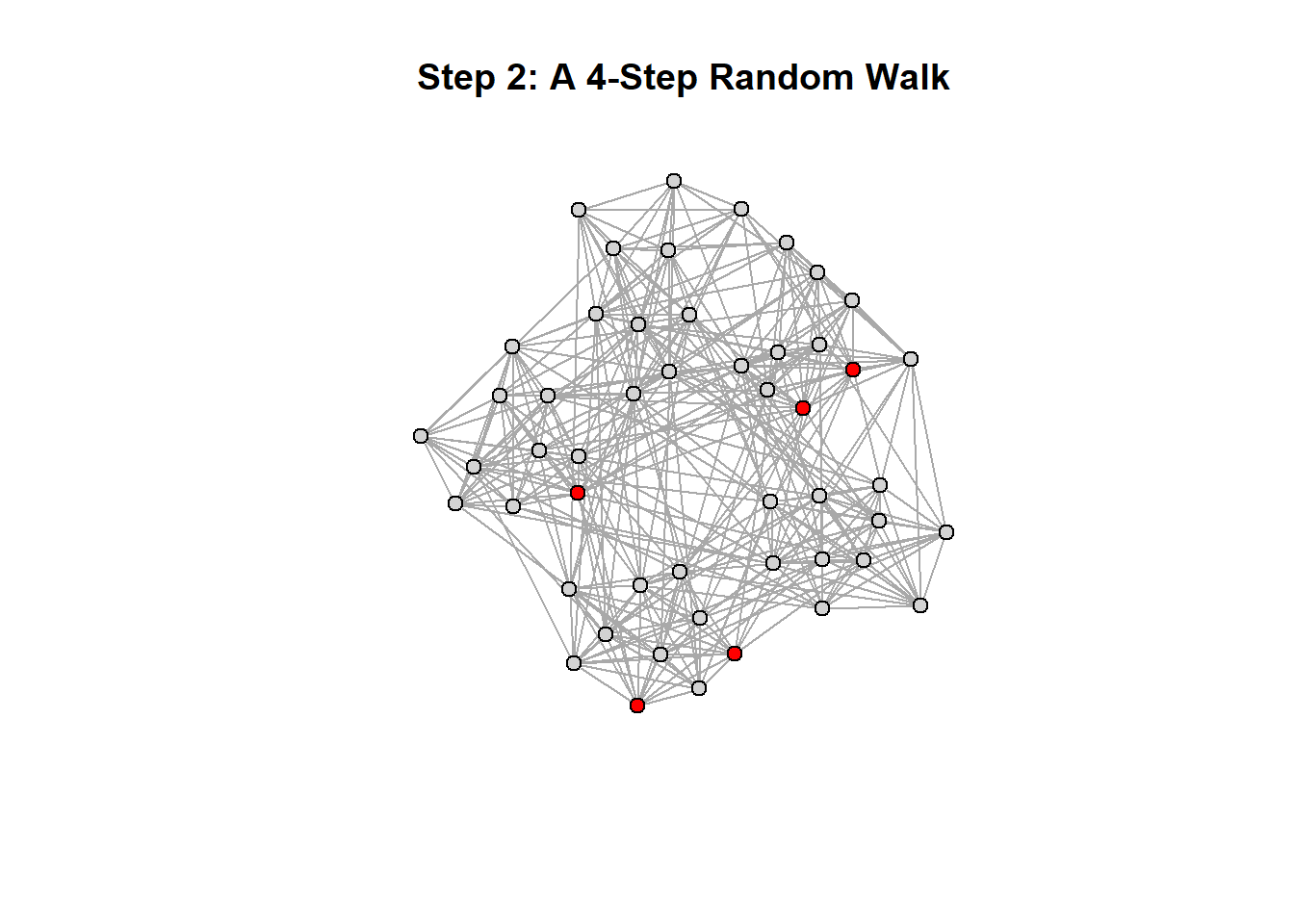
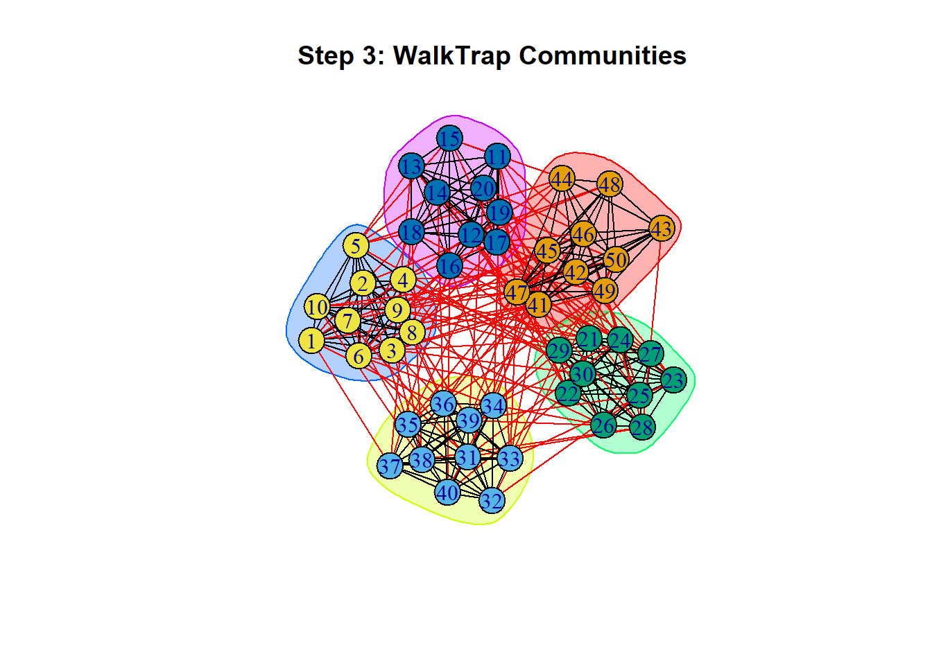
WalkTrap is a community detection method based on random walks on the network. For example, if you walk 4 steps from any node, where do you end up? If another node takes 4 steps, where would they end up? If both nodes ended up in the same place, doesn’t that mean they are close enough to be in the same community?
By default, this is metric is measured in 4 steps walks, but where do we think “good” cutoffs should be? What happens if we add or subtract steps?
The entire idea of WalkTrap is about maximizing the amount of ways you can get to neighboring nodes so that two nodes end up in the same place. With a default of 4 steps, random walks are simulated in WalkTrap and nodes with similar walk distributions are grouped together in the same community (Pons and Latapy (2005); Gates et al. (2016)).
None of these metrics are infallible indicators of how amazing your partitions are. There is always nuance and checking the assumptions of each test and what you are looking for is highly important.
----------------------------------------------------
Gaussian finite mixture model fitted by EM algorithm
----------------------------------------------------

Mclust EII (spherical, equal volume) model with 5 components:

 log-likelihood  n  df       BIC       ICL
      -1982.977 50 255 -4963.519 -4963.519

Clustering table:
 1  2  3  4  5
10 10 10 10 10
[1] 1 1 1 1 1 1 1 1 1 1 2 2 2 2 2 2 2 2 2 2 3 3 3 3 3 3 3 3 3 3 4 4 4 4 4 4 4 4
[39] 4 4 5 5 5 5 5 5 5 5 5 5 Spectral k.Means c.Means GMM WalkTrap
1 1 1 1 1 1After running all our metrics, we can see that 5 clusters is the best amount of clusters without over-fitting or forcing clusters and that all methods of validation agreed on this. If we were truly writing a paper describing our network, we would have to choose the right metric(s) that appropriately match the data, have assumptions that we are aware and approving of, and are cognizant of the limitations of the metric(s) we chose.
In many psychological and behavioral data sets, networks are constructed from correlations or partial correlations rather than direct interactions. This introduces an important conceptual difference: edges no longer represent discrete events or connections, but statistical associations (Brusco, Steinley, and Watts (2024b); Brusco, Steinley, and Watts (2024a)). A core, technical challenge is that statistical associations in correlation matrices are mathematically inconsistent with the null models of community detection (MacMahon and Garlaschelli (2013)).
Using the psychological example of building networks of symptoms into diagnoses, the edges are representing associations between symptoms in an attempt to explain the structure of diagnoses. However, we need to stop and think about what it actually means to detect a “community” in these types of networks.
Using the partial correlation basis of psych networks, all nodes are indirect and statistical and to some degree are all connected. This opens questions such as what does it mean for two nodes to be “close”? Does this mean that symptoms share mechanisms or, going up a level, that seemingly differentiated diagnoses share symptoms and are “related”?
All the questions that arise from the nature of psych networks all center on the nature of correlational clusters and the problems they present. Correlation-based networks do not hold the assumptions of clear separation between groups, meaningful distances and connections between nodes, and the very relationships between nodes are unstable and are questioned. This can result in high degrees of overlapping, fuzziness, and inaccurate clustering. As Park, Chow, and Molenaar (2024) lays out, symptoms start to act like “bridges” between communities, forcing nodes into discrete groups, which may be inaccurate and bias results.
This suggests that the goal of clustering in these contexts is not necessarily to identify “true groups,” but to explore structure, identify patterns, and generate hypotheses—while remaining cautious about interpretation.
To close, being aware of the assumptions underlying cluster quality metrics, visualization methods, and the structure of the graph itself is critical. While network analysis offers powerful tools for uncovering patterns, applying these methods without careful consideration can lead to misleading or overstated conclusions. Thoughtful application is therefore just as important as the methods themselves.