What are “Psychological” Networks? (Fried, 2020 & Epskamp et al., 2017 & Borsboom & Cramer, 2013)
A dominant paradigm used in modeling psychopathology is the latent variable framework, or the common cause model. This is heavily inspired from how western medicine models their own diseases. The way we handle and collect psychopathological data is also greatly influenced by this approach. We can describe this approach as follows:
Imagine someone comes to a hospital presenting with chest pain, shortness of breath, and coughing up blood. These symptoms can be caused by a lung tumor.
In psychology, someone can present with sleep problems, depressed mood, and suicidal ideations. These symptoms can be caused by Major Depression (MD)
However, a major difference between this medical model and the behavior of psychopathological disorders is that mental disorders themselves are not empirically identifiable and cannot be diagnosed independent of their symptoms.
For example:
One may feel chest pain without having a lung tumor. One may also have a lung tumor without feeling any chest pain. Think of the early stages of the tumor; one could have a lung tumor without feeling any symptoms at all.
In psychopathology, one cannot have, say MD, without experiencing symptoms of MD. In other words, mental disorders cannot be separated from their symptoms, and therefore, cannot by causes of their symptoms.
This relationship between mental disorders and their symptoms being inseparable leads to the need for a different way of conceptualizing and modeling these constructs. One where perhaps mental disorders are in fact a system caused by the activation of symptoms.
The psychological network approach provides a new framework for understanding different psychological constructs (i.e. depression, anxiety, PTSD, etc.). Alternative approaches such as latent variable models consider things like symptoms, behaviors, or emotions as an indication of an underlying disorder/psychological construct. Psychological networks on the other hand, considers all of these symptoms as individual interacting variables in their own right that together describe a psychological construct.
This figure is from Lack of Theory Building and Testing Impedes Progress in The Factor and Network Literature (Fried, 2020). “PC” indicates Psychological Construct.
Why do we use partial correlations? (Williams et al., 2019 & Borsboom et al., 2021 & Eskamp et al., 2018)
A goal of psychological network analysis is to model direct pathways/connections between variables (something the latent variable framework can’t do).
Partial correlations answer which symptoms influence each other once everything else is accounted for.
A network composed of partial correlations estimates a sparse network of conditional relations (i.e. direct connections) from the observed variables.
Any correlation matrix, \(\mathbf{\Psi}\) may be converted into a set of partial correlations using the precision matrix, \(\mathbf{K} = \mathbf{\Psi}^{-1}\), where:
elements of K being standardized \[P_{ij} = -\frac{\kappa_{ij}}{\sqrt{\kappa_{ii}\kappa_{jj}}}\]
Basically:
we have a correlation matrix, \(\mathbf{\Psi}\), that is obtained from the data
this correlation matrix is inverted, resulting in the precision matrix \(\mathbf{K} = \mathbf{\Psi}^{-1}\)
the different elements of the precision matrix \(\mathbf{K}\) are plugged in to the equation above to obtain partial correlations.
if \(\kappa_{ij}\) = 0, the partial correlation is 0 and no edge connection is made between these elements
if \(\kappa_{ij} \neq\) 0, the partial correlation is non-zero, and an edge connection is made. Meaning these elements have a conditional relationship after controlling for all other variables
Alternatively, it can be calculated in matrix form by defining a diagonal matrix, \(\mathbf{D} = \text{Diag}(\mathbf{\Psi})\) and \(\mathbf{I}\) is the identity matrix:
Both of these result in identical results but the latter is a matrix form of the former.
Before moving on:
Is “sparsity” something we expect in reality? Is this assumption realistic, especially in a psychological context?
Psychological processes are incredibly interconnected, even if some of those connection may be weak, they could very likely still be real. From the readings, it seems there is a trade-off between sensitivity and specificity, detecting edges and false positive rates. Also, for the purposes of interpretation and stability.
Recall: the goal is to create conditional relationships. What happens if we add one more variable to the network? Or remove one?
Conditioning for other things means that all relations change when you include even a single new variable. Every time you add or remove a variable (node), the partial structure will change.
More on Sparsity and Partial Correlations
We are trying to estimate a sparse network. However, the partial correlation matrix does not enforce sparsity.
Below, I read in a raw correlation matrix that has \(40\%\) sparsity and then convert the correlation matrix into a partial correlation matrix using the equations above.
Note in the correlation matrix below, we do observe sparsity but in the conversion to a partial correlation matrix, sparsity is not preserved.
# Setup Psi =round(readRDS("./excor.RDS"), 2) # the covariance matrix K =solve(Psi) #compute the inverse of the covariance matrix. AKA precision matrix D =diag(K) #Contains all diagonal elements of matrix D.root =diag(1/sqrt(D)) #Square root of those diagonal elements (the denominator of the partial correlation equation) pcor.slow =matrix(NA, nrow(Psi), ncol(Psi)) #empty matrix for the partial correlations# Equation 1for(i in1:nrow(K)){for(j in1:ncol(K)){ pcor.slow[i,j] =-K[i,j] / (sqrt(K[i,i] * K[j,j])) #this is the equation above } }round(pcor.slow, 2) #what do we see in the results? No more 40% sparsity in the partial correlation matrix
Every partial correlation value is non-zero, indicating many (be it strong or weak) connections between nodes. Therefore, indicating a dense network.
Purpose of Regularization (Epskamp et al., 2017 & Epskamp et al., 2018 & Williams et al., 2019)
Partial correlations quantify conditional relationships between variables, but they do not inherently produce sparse networks. Sparse psychological networks are imposed only when regularization methods such as the graphical LASSO are applied to shrink many partial correlations to exactly zero.
Statistical purpose
Regularization is used to estimate network model parameters (i.e. the precision matrix). This is especially helpful in high-dimensional settings where the number of variables (p) is approaching or exceeds the sample size (n). This approach is useful in noisy settings where one wants to be more conservative in detecting (spurious) edges and a lower false positive rate. This method works best when the “true” network is sparse.
Most commonly employed is the LASSO method (for networks: glasso with an EBIC determined tuning parameter).
The objective function for LASSO on a simple linear regression:
\(\sum\limits_{i=1}^{n} (y_i - \sum_j x_{ij}\beta_j)^2\) is the model fit/linear regression
and
\(\lambda \sum\limits_{j=1}^{p}\lvert\beta_j\rvert\) is the penalty term
Both lasso and glasso shrink parameters toward zero based on their penalty term. Lasso shrinks regression coefficients and glasso shrinks elements of the precision matrix. For glasso, EBIC is commonly used to determine the strength of the penalty. A stronger penalty encourages a sparser network.
Empirical purpose
Regularization shrinks many weak edges to zero, thus producing a sparse network. This is beneficial from a theoretical standpoint because, if every variable in a psychological network were connected, then we would learn nothing about which relationships are directly important.
Does regularization align with our conceptual understanding of real-world psychology?
Is reality sparse?
Limitations of Regularization
Regularization assumes sparsity and forces partial correlation values to zero. However, this doesn’t seem to be a valid assumption especially in regards to psychological constructs. It is likely that in the endeavor to obtain sparsity, we are missing many real connections between nodes.
Additionally, the benefit of regularization in high-dimensional settings (high p and low n) is not typically the case in psychology. We actually tend to find ourselves in the situation of p << n.
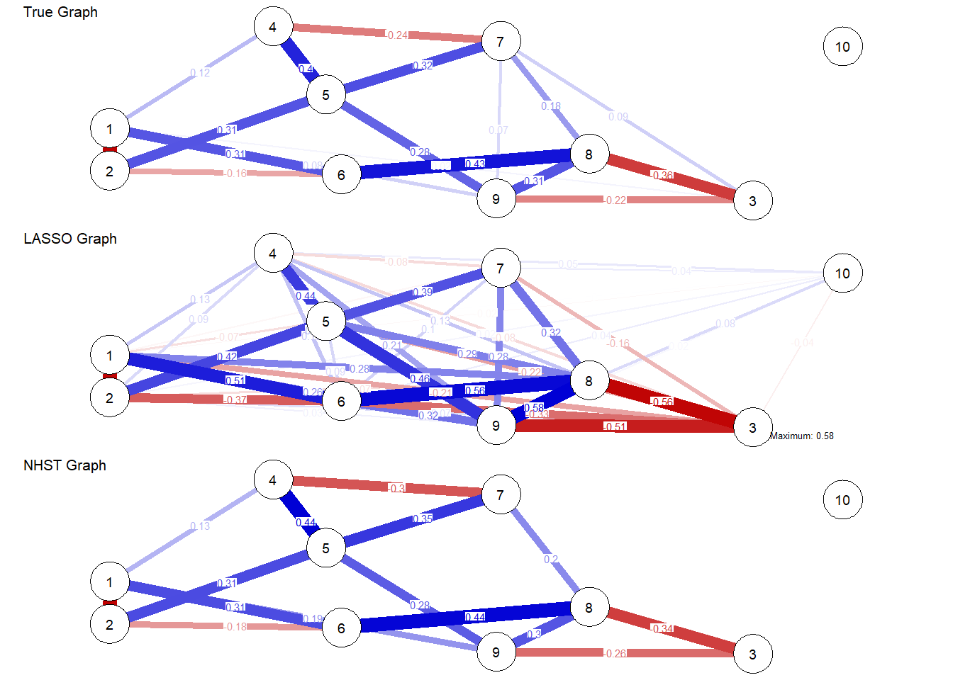
Alternative methods that don’t use regularization have been shown to perform better than the glasso, such as low-rank approximation and NHST Gaussian Graphical Modeling.
library(GeneNet)
Loading required package: corpcor
Loading required package: longitudinal
Loading required package: fdrtool
library(qgraph)library(GGMnonreg)
Registered S3 method overwritten by 'GGMnonreg':
  method     from
  plot.graph GGMncv
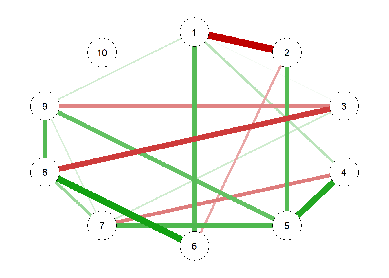
library(rlang)set.seed(89181)# Generating True Model true.pcor =ggm.simulate.pcor(num.nodes =10, etaA =0.40) #what percent of edges should be non-zero# qgraph(true.pcor, edge.labels = TRUE)# Generating Data From Model m.sim =ggm.simulate.data(sample.size =600, true.pcor)## Covariance implied by Data CovMat =cov(m.sim)# Modeling the true correlations G1 =qgraph(true.pcor)
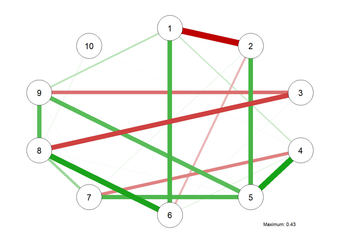
# Estimating the EBIC Graphical LASSO Network Model EBICgraph =qgraph(CovMat,graph ="glasso",sampleSize =nrow(m.sim),tuning =0.50,details =TRUE)
Warning in EBICglassoCore(S = S, n = n, gamma = gamma, penalize.diagonal =
penalize.diagonal, : A dense regularized network was selected (lambda < 0.1 *
lambda.max). Recent work indicates a possible drop in specificity. Interpret
the presence of the smallest edges with care. Setting threshold = TRUE will
enforce higher specificity, at the cost of sensitivity.
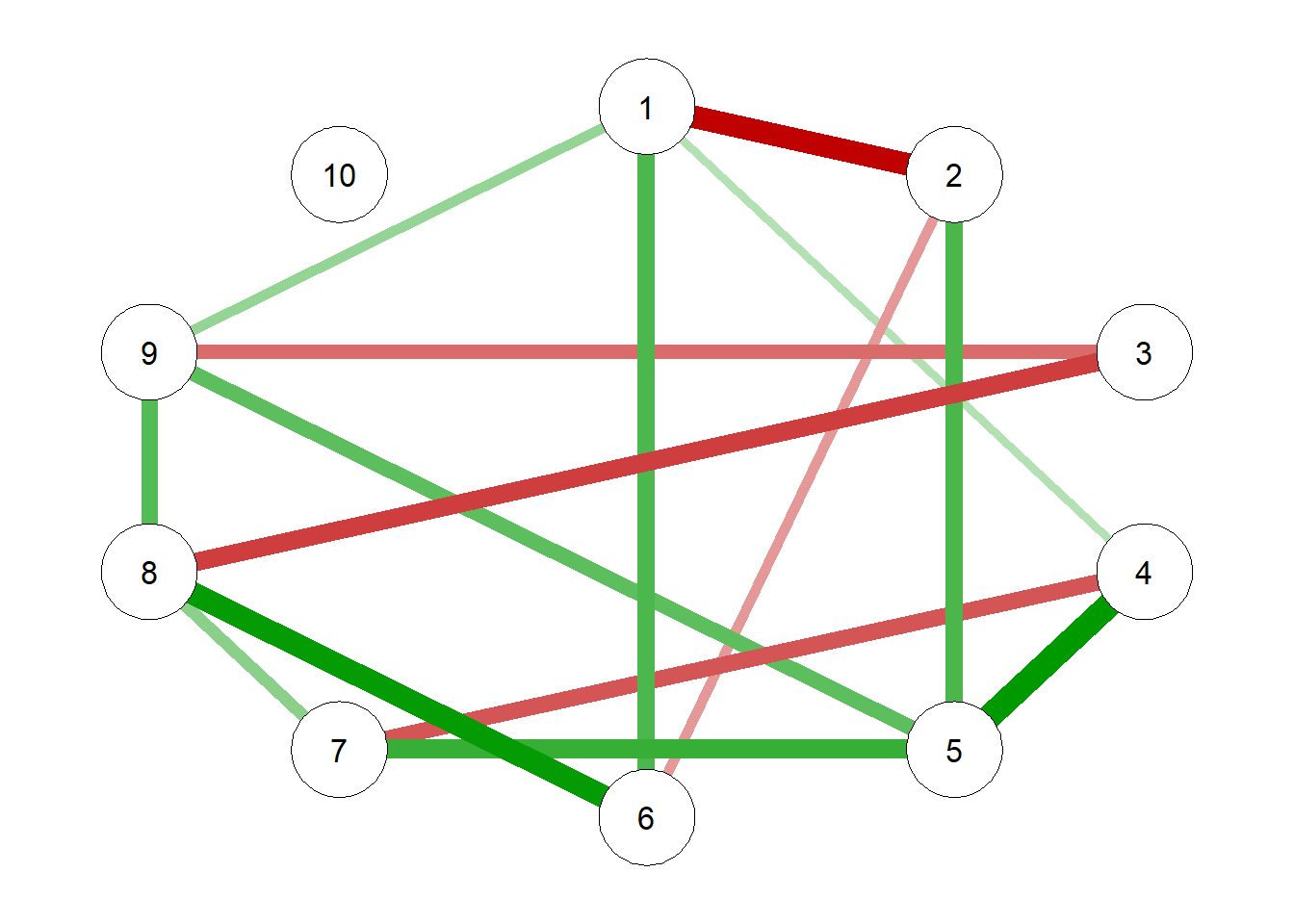
# EBICgraph = qgraph(MyData, graph = "glasso", sampleSize = nrow(m.sim), tuning = 0.50, details = TRUE)# Estimating the NHST Gaussian Graphical Model and Generating a Plot; Williams et al,# Does not have shrinkage as an issue NHSTgraph =ggm_inference(m.sim, alpha =0.05)
# Network Comparison Testlibrary(NetworkComparisonTest) true.pcor1 =ggm.simulate.pcor(num.nodes =10, etaA =0.20) #fewer but stronger edges true.pcor2 =ggm.simulate.pcor(num.nodes =10, etaA =0.50) #more but weaker edges m.sim1 =ggm.simulate.data(sample.size =100, true.pcor1) m.sim2 =ggm.simulate.data(sample.size =100, true.pcor2)# Elaborating on options and results; in this case, networks differ:# In structure but not in global strengthNCT(m.sim1, m.sim2, it =2000)
 NETWORK INVARIANCE TEST
 Test statistic M:
 0.7313794
 p-value 0.0004997501

 GLOBAL STRENGTH INVARIANCE TEST
 Global strength per group:  4.736806 2.810594
 Test statistic S:  1.926212
 p-value 0.189905
# NCT(m.sim1, m.sim1, it = 2000)
What characteristics do “psychological” networks tend to have that networks in other fields do/do not have?
On a similar note of limitations …
Psychological networks are undirected. The edges in these networks represent conditional relationships, not causal directions. This is different from say a social network where for example we can represent that “person A” befriended “person B” and “person C” befriended “person D.”
Assigned edge weights (partial correlations) are bounded between -1 and 1. These weights are linked to each other and must create a valid positive-definite precision matrix.
a =matrix(c(1, 0.99, 0,0.99, 1, 0.99,0, 0.99, 1), 3, 3)eigen(a)
#We need the eigen values to be be positive. Here, one is negative therefore this is not a valid correlation matrix. This is caused by the 0's in the matrix. The high surrounding correlation values would require the zero elements to also be high values in order to be considered a valid correlation matrix.
a =matrix(c(1, 0.99, 0.97,0.99, 1, 0.99,0.97, 0.99, 1), 3, 3)eigen(a)
The edges in psychological networks are estimated, not observed. They can vary depending on how you estimate them, sample size, number of variables, use of regularization, etc. Compare this to say in a social network for example, edges can be created from “person A” to “person B” via reported friendship statuses (i.e. survey responses).
Given all we have gone over, what are some thoughts regarding these types of “networks”. What are their strengths? Are there other limitations in regards to discussions we’ve already had throughout the quarter? (Hint: think about Modularity and Centrality measures)
Due to these differences (non-direction, constrained weights, estimation of edges), many commonly used network metrics no longer work or no longer mean the same thing because their assumptions have been violated. Modularity assumes observed independent edge weight, which is violated by constrained partial correlation estimates. Betweenness and closeness centrality depend on shortest paths, which become difficult to determine when regularization removes edges or when estimation errors alter paths.
Typically we create psychological networks from items that were originally made to measure latent variables. This makes for highly similar and correlated nodes in the network. This is a problem, because these redundant nodes will compete to explain the same variance, this will weaken the meaningful connections between other nodes. For example, say “node A” and “node B” are meaningfully connected. Adding a duplicate of node A, “node A2” (a node that will be highly correlated to node A), will weaken the connection between “node A” and “node B.”
The point of psychological networks is to model direct relationships between different variables/symptoms. Conceptually it allows these symptoms to interact with each other (unlike in a latent variable framework). These networks do still support strength centrality metrics (Bos et al, 2017). Psychological networks can also be extended to time-series networks (VAR/GVAR models) (Epskamp et al., 2018).
How can we gather psychological data to better reflect the networks in other fields?
What about co-occurrence; Probabalistically one could do an Ising model (binary model) (Van Borkulo et al., 2014 & Haselbeck et al., 2021)