At the beginning of this course, we learned the most basic form of a graph, the simple undirected graph. It’s the one given by G = (V, E) Where: G: the graph… is given by V: a set of vertices… and E: in plain English, is the subset of {x, y}, pairs of vertices which are connected to one another (they’re edges)
What are their shortcomings?
So far, we’ve been learning about networks as if all connections exist at the same time and have always been present, and this is called a “static” network. But, in real life, connections don’t just start to exist all at once, they form and fade away over time, like synaptic connections in the brain that are pruned or lost to damage and re-routing, or friends who come into our lives and leave.
When we compress a network into one static picture, we ignore the order of events. Not knowing the temporal sequencing (timing) of events can result in erroneous directional interpretations (inaccurate representations of the order stuff happens in). For example:
library(sna)
Loading required package: statnet.common
Attaching package: 'statnet.common'
The following objects are masked from 'package:base':

    attr, order
Loading required package: network
'network' 1.19.0 (2024-12-08), part of the Statnet Project
* 'news(package="network")' for changes since last version
* 'citation("network")' for citation information
* 'https://statnet.org' for help, support, and other information
sna: Tools for Social Network Analysis
Version 2.8 created on 2024-09-07.
copyright (c) 2005, Carter T. Butts, University of California-Irvine
 For citation information, type citation("sna").
 Type help(package="sna") to get started.
library(tsna)
Loading required package: networkDynamic
'networkDynamic' 0.11.5 (2024-11-21), part of the Statnet Project
* 'news(package="networkDynamic")' for changes since last version
* 'citation("networkDynamic")' for citation information
* 'https://statnet.org' for help, support, and other information
library(ndtv)
Loading required package: animation
'ndtv' 0.13.4 (2024-06-30), part of the Statnet Project
* 'news(package="ndtv")' for changes since last version
* 'citation("ndtv")' for citation information
* 'https://statnet.org' for help, support, and other information
n_nodes =max(c(df$tail, df$head)) base_net =network.initialize(n_nodes, directed =FALSE)# The dataframe should be turned into a Temporal Network: net_dyn =networkDynamic(base.net = base_net,edge.spells = df[, c("onset", "terminus", "tail", "head")])
Created net.obs.period to describe network
 Network observation period info:
  Number of observation spells: 1
  Maximal time range observed: 10 until 300
  Temporal mode: continuous
  Time unit: unknown
  Suggested time increment: NA
coord <-network.layout.fruchtermanreingold(network.extract(net_dyn, at =1), NULL)
Element of Time
The fix? Introducing time.
Instead of asking “are nodes connected?” we want to ask “can information actually travel through these connections?” Only by adding time do we correctly see what sequences of influence are actually possible.
All of this matters because by ignoring time, relationships look more flexible than they are and paths may look possible but not actually be possible. This is why we need to represent networks in a way that keeps track of when things happen, not just whether they happen.
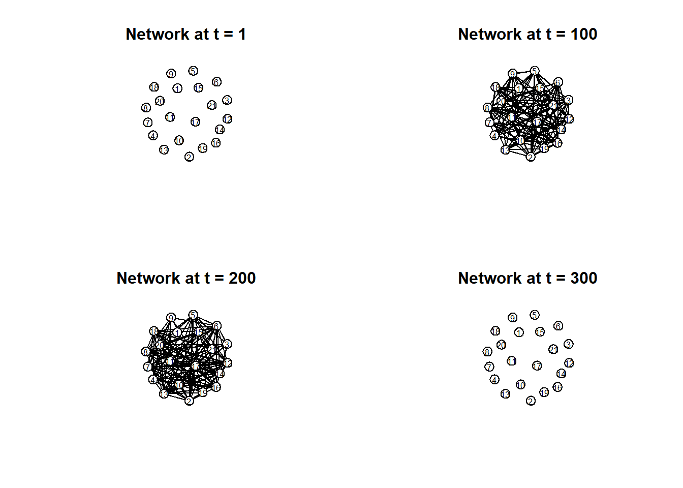
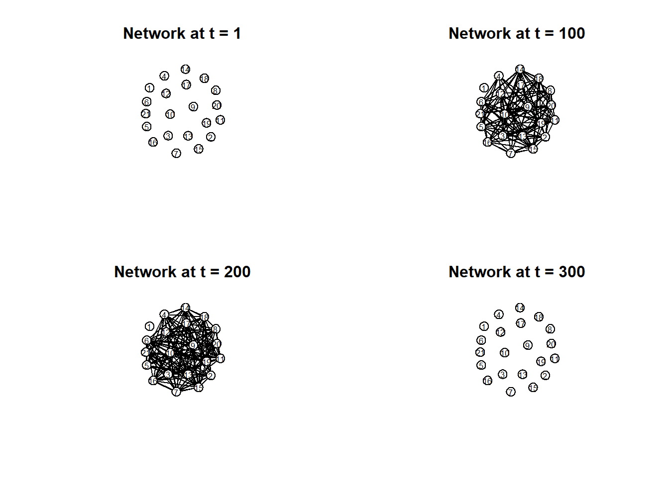
# Plot separate moments in time:par(mfrow =c(2, 2)) times =c(1, 100, 200, 300) titles =paste("Network at t =", times)invisible(lapply(seq_along(times), function(i) {plot(network.extract(net_dyn, at = times[i]),main = titles[i],displaylabels =TRUE,label.cex =0.6,label.pos =5,vertex.col ='white',vertex.cex =5,coord = coord) }))
Introducing …
Temporal Networks!
G (V, E) Where: G: the graph… is given by V: a set of vertices… and E: the subset of {x, y}, pairs of vertices which are connected to one another but are not the same vertex (x does not = y)
Now, we meet G (V, E, D) Where: D is a “dimension” of the network representing different layers. Each layer is a “slice” of time
D is a dimension that can be added to represent lots of other things like weights, probabilities, and categories. In the specific multilayer network we will be learning about, D represents time.
Temporal Closeness and Efficiency
# Temporal Closeness and Efficiency calc.temporal.closeness =function(net.dyn, start =NULL) { n =network.size(net.dyn)if (is.null(start)) start =min(df$onset, na.rm =TRUE)sapply(1:n, function(i) { tp =tryCatch(tPath(net.dyn, v = i, direction ="fwd", start = start), error =function(e) NULL)if (is.null(tp)) return(0) d = tp$tdist[is.finite(tp$tdist) & tp$tdist >0]if (length(d) ==0) return(0)mean(1/ d) }) } calc.temporal.efficiency =function(net.dyn, start =NULL) {mean(calc.temporal.closeness(net.dyn, start = start), na.rm =TRUE) }calc.temporal.closeness(net_dyn, start =10)
One of the topics we discussed was closeness centrality, which asks how close one node is to all other nodes based on the shortest path. But In temporal networks, we redefine closeness using time-respecting paths.
As we read in the paper by Pan and Saramaki, temporal closeness is based on the earliest time that information can travel from one node to another, instead of the fewest steps. It is about the fastest feasible journeys through time, not the shortest structural path.
Static closeness is still useful as a baseline, telling us who is structurally central, but doesn’t say much about how efficiently things spread in reality.
Another key concept discussed in the Holme & Saramaki paper is reachability, describing how, in a temporal network, node A is reachable from B if there’s a sequence of time ordered interactions that allows information to travel from B to A. This is different from a simple di-graph because if there’s a path A—>B—>C, we say A can reach C but in a temporal network, that path only matters if the edges occur in the correct order in time. Structure alone is not enough because causality requires time-respecting paths.
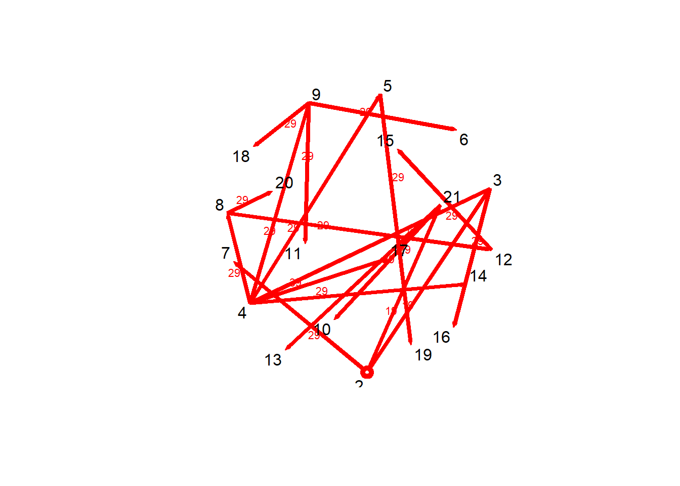
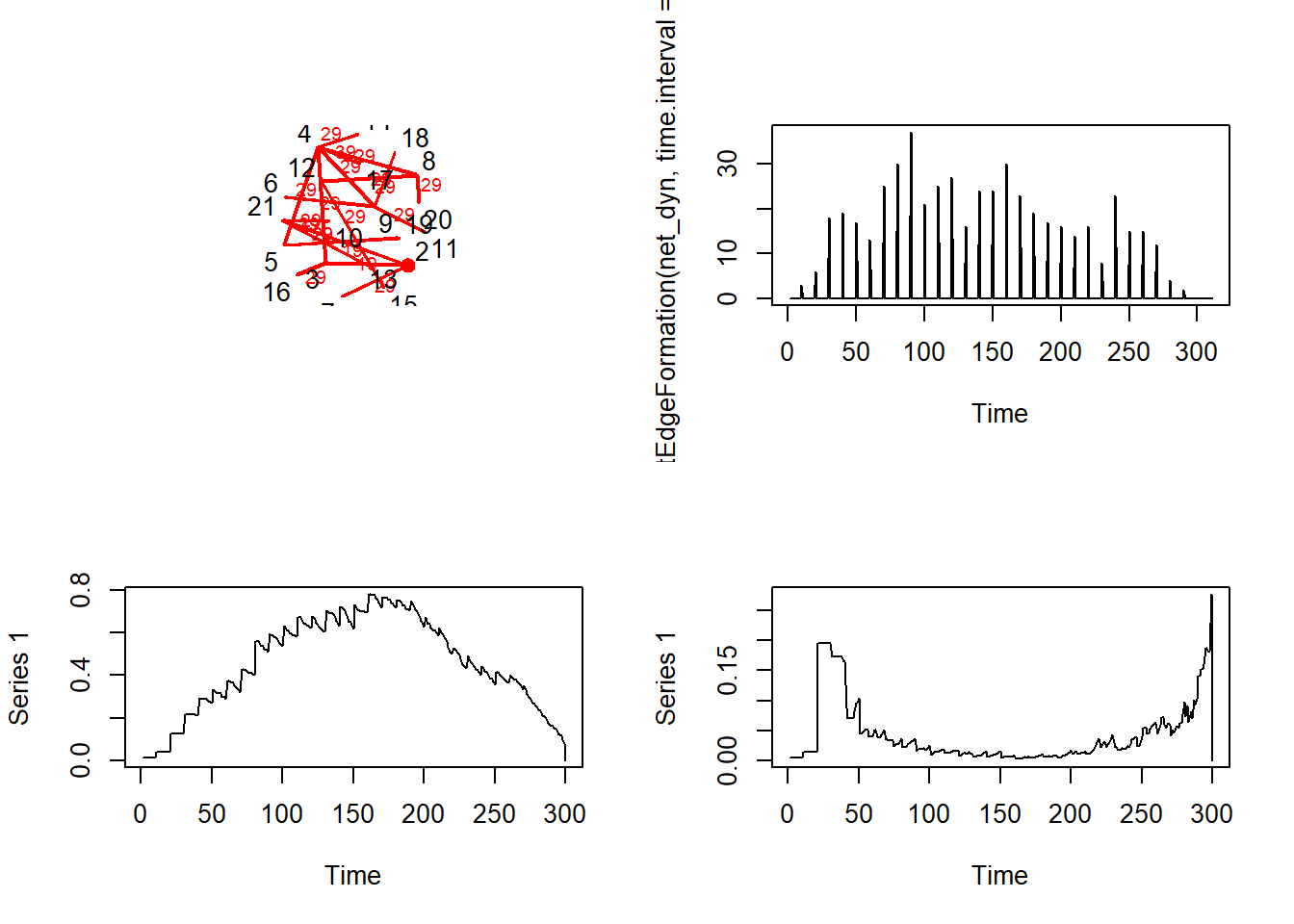
# tdist: distance from t = origin for v to affect the i^{th} node# previous: The node that immediately preceeded landing on the i^{th} node# gsteps: The number of "graph" steps to get to the i^{th} nodeplot(v1path, coord = coord,displaylabels =TRUE)
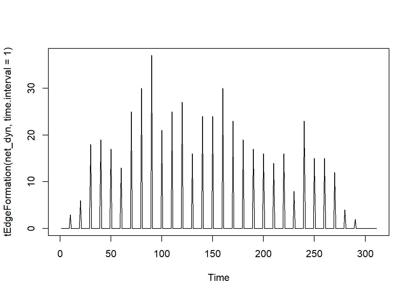
# Observing the number of connections as a function of timeplot(tEdgeFormation(net_dyn, time.interval =1))
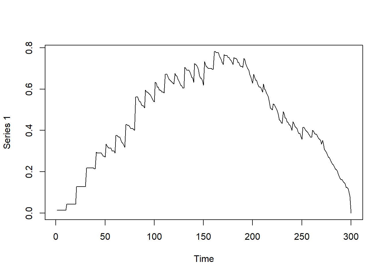
# Observing graph-based density as a function of time dynamicdensity =tSnaStats( net_dyn,snafun ="gden",start =1,end =300,time.interval =1,aggregate.dur =10 )plot(dynamicdensity)
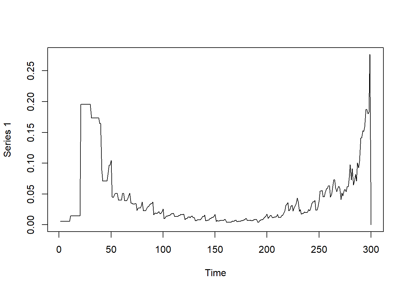
Observing betweenness in the graph over time
# Observing betweenness in the graph over time dynamicbtw =tSnaStats( net_dyn,snafun ="centralization",start =1,end =300,time.interval =1,aggregate.dur =10,FUN ="betweenness" )plot(dynamicbtw)
Introduction to Dynamic Networks
In contrast to the temporal network, where edges appear and disappear over time, a dynamic network is a bit broader. A dynamic network–for this class–is considered some form of model fitted to time-series observations The temporal network focuses on the timing of interactions while the dynamic network focuses on the evolution of the network. The parameters of a dynamic network can describe how the system behaves on an average over time. The parameters represent the steady-state dynamic The nodes can represent the measured variables of individuals such as symptoms moods or personality traits The edges can represent the strength and relationships between nodes Describes how the system fluctuates between its typical state Example: A sucidial individual who normally keeps to themselves. Starts to visit family and friends every Friday night. The family and friends are pleasantly surprised and even say “It’s so great to spend time with you, we typically dont hear from you often.” Until days later wher that individual goes back to spending Friday nights by themselves.
What are some popular dynamic network “models”
Dynamic networks use various types of statistical techniques. One of which is the Vector Autoregression.
The Vector Autoregression (VAR)
Simply: A way to model multiple time series that influence each other over time. Each variable depends on its own past and the past of the rest of the variables. The core components: Quantifies lagged effects where the previous degree of one variable can predict the next variable from previous times Cross-lagged effect: one variable predicts predicts another variable at next time point Ex: Anxiety today → Sad tomorrow Autoregression, can show a variable be predicted at the next measurement. A high autoregression may suggest where the baseline is likely to slowly return. Present same variables correlated with each other EX: Sad today → Sad tomorrow
\[\mathbf{\eta_{t}} = \mathbf{\Phi}\eta_{t-1} + \mathbf{\zeta}_{t}\] where \(\mathbf{\eta}\) represents a \(p\)-variate vector of scores on our latent variables, \(\mathbf{\Phi}\) represents our \(p\times p\) regression coefficients matrix relating past scores on our latent variables with current scores, and \(\mathbf{\zeta}\) is our \(p\)-variate vector of residuals \(\{\mathbf{\zeta}\} \sim \text{WN}(0, \mathbf{\Psi})\) and \(\mathbf{\Psi}\) is the \(p\times p\) matrix of innovation covariances. > Breakdown: nt: current latent state, a list of your latent variable scores at time t (where the system is now) nt-1: previous latent state, the same variables, but one time unit earlier than nt (where the system just was at previously) t - 1: known as the first lag Circle with the I (Phi): Tells you how one variable at time t-1 influences another at time t, or a transition matrix Zeta t: process the “noise” with specifically two random variables being measured to indicate the direction of the relationship.
##The Graphical and Structural VAR
Both the GVAR and SVAR focus on contemporaneous relationships: how variables influence each other within the same time point, rather than across time like lagged effects (lagged effects is what we talked about before, VAR, where the past variables affect variables at a later point in time) Example: You complain to a friend that you have a terrible headache, and they hand you a pain realiver to alleviate the headache. After 5 hours the friend checks up on you and ask you if the medication they gave you helped, and you still feel a pounding pain on your temples so you say “Sadly no” The reasoning behind this effect is that the medication didnt get fully metabolize, and your headache still appear. After another period of time, the medication starts to take effect and your headache disappears
Both of these models look at “contemporaneous” or “faster” dynamical features than our lagged effects.
The GVAR
Using the VAR model, gVAR similarly uses multiple models to understand how variables influence each other over time and how they relate to each other in the exact same moment. gVAR is also a non-directional network that helps identify the simultaneous associations between variables. In other words, gVAR helps filter the noise (residuals) of variables that VAR couldn’t explain. Ex of VAR: Stress yesterday → Stressed today gVAR: Stress today - Mood today
The SVAR
The structural VAR tries to answer, “What variable causes another variable to react in present time”. sVAR tries to separate variables to assign direction and interpret A and B influences. sVAR is an extension or reformulation of VAR but sVAR adds on by explaining the contemporaneous relationships affects other variables in current time other than focusing on the lagged effects Ex of VAR: Happy yesterday → Happy today sVAR: current anxiety → current mood
Slightly different model notation:
\[\mathbf{\eta_{t}} = \mathbf{A}\eta_{t} + \mathbf{\Phi}^{*}\eta_{t-1} + \mathbf{\zeta}_{t}^{*}\] where \(\mathbf{A}\) represents a \(p\times p\) matrix of contemporaneous effects with \(0\)’s along the diagonal, \(\mathbf{\Phi}^{*}\) is the \(p\times p\) matrix of lagged effects, and \(\mathbf{\zeta}^{*}\) is the \(p\)-variate vector of residuals assumed normally distributed with an identity covariance, \(\{\mathbf{\zeta}^{*}\} \sim \text{WN}(0, \mathbf{I}_{p})\). > n(t): The time in which variable occurred An(t): same-time(contemporaneous) effects at time (t) Phi n(t - 1): the relationship dependent relationship between variables and the directed measurement of time. (The p x p matrix) Zeta(t): The errors commonly assumed or the residual vector that process the “noise”
As far as you can tell, how are they similar or different?
sVAR vs. gVAR
gVAR: - Non-directional, can infer relationships between variables but not give a clear connected relationship - partial correlation relationship
sVAR: - Shows influence on variables and direction varies on influence between variables - Directional(but with certain warnings that depend on the direction of the variable) “The direction of the variables exist”
Solution found! Final fit=30876.743 (started at 35815.467) (1 attempt(s): 1 valid, 0 errors)
Start values from best fit:
0.532197082221117
summary(ar1)$parameters
          name matrix row col  Estimate   Std.Error lbound ubound lboundMet
1 OUMod.A[1,1]      A   1   1 0.5321971 0.007572714     NA     NA     FALSE
  uboundMet
1     FALSE
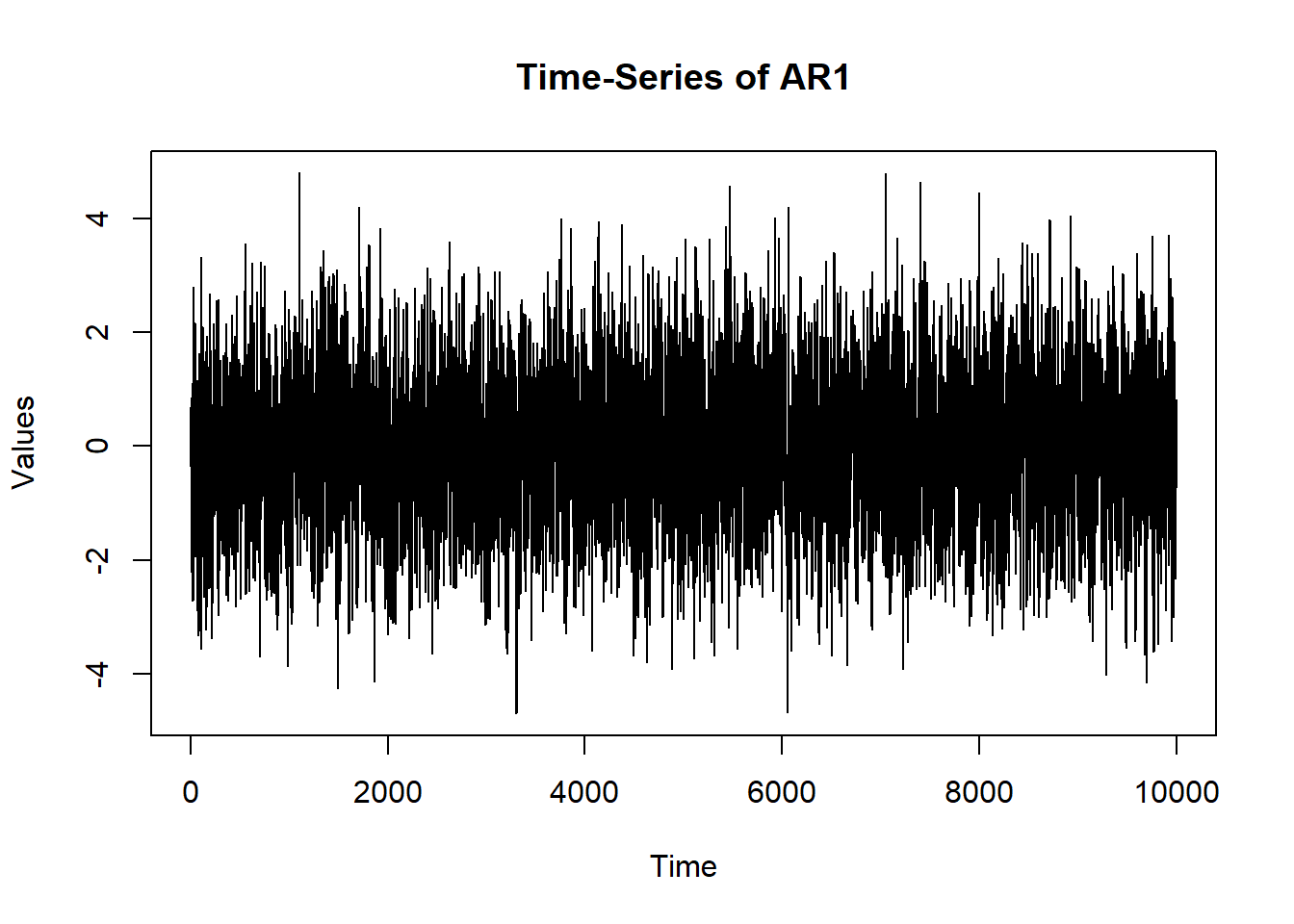
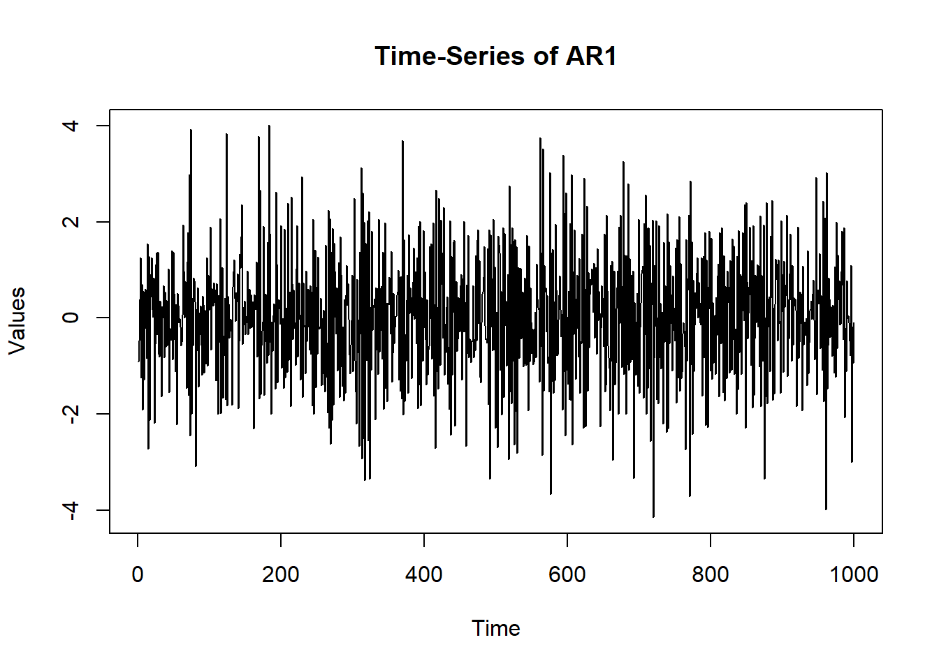
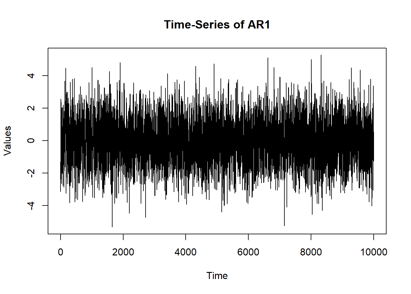
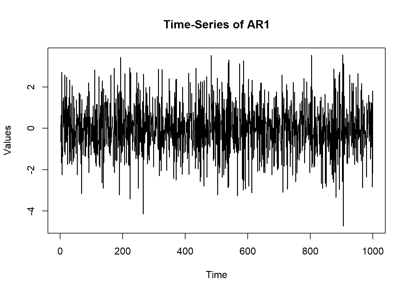
# Can compare to different AR: osc$A$values =-0.60 sim.data =mxGenerateData(osc, nrows =1000)plot(x = (1:nrow(sim.data)), y = sim.data$AR1, type ="l",main ="Time-Series of AR1", ylab ="Values", xlab ="Time")
          name matrix row col    Estimate  Std.Error lbound ubound lboundMet
1 OUMod.A[1,1]      A   1   1  0.57113567 0.02411648     NA     NA     FALSE
2 OUMod.A[2,1]      A   2   1  0.05460886 0.02411601     NA     NA     FALSE
3 OUMod.A[3,1]      A   3   1  0.02609933 0.02412602     NA     NA     FALSE
4 OUMod.A[1,2]      A   1   2  0.02647079 0.02625484     NA     NA     FALSE
5 OUMod.A[2,2]      A   2   2  0.59992109 0.02625472     NA     NA     FALSE
6 OUMod.A[3,2]      A   3   2 -0.24751145 0.02626571     NA     NA     FALSE
7 OUMod.A[1,3]      A   1   3  0.22289384 0.02416879     NA     NA     FALSE
8 OUMod.A[2,3]      A   2   3 -0.02662749 0.02416713     NA     NA     FALSE
9 OUMod.A[3,3]      A   3   3  0.58643686 0.02417257     NA     NA     FALSE
  uboundMet
1     FALSE
2     FALSE
3     FALSE
4     FALSE
5     FALSE
6     FALSE
7     FALSE
8     FALSE
9     FALSE
You are a highly exclusive detective attending a charitable Gala on Friday the 13th with a total of 450 guests in attendance. Which contains 150 A-list celebrities, 150 politicians, and 150 billionaire tycons who plan to auction off the incredibly expensive and irreplaceable Pink Panther Diamond!
Your comrades are: VAR an undercover detective with sVAR and gVAR, the junior undercover detectives.
Throughout the gala You, VAR and sVAR interact with party guests and gather information on who they are, how they are feeling, and plans for tomorrow. Important side note, VAR is keeping track of time for the numbered interactions, and takes occasional social breaks throughout the Gala. While gVAR sits in the corner unimpresingly observing and analyzing everyone’s emotion and behavior. Overall, every VAR is accounting for time as they attend the gala. As day enters the night, everyone’s mood drops, as a famous billionaire politician gets murdered in the Ballroom! Shocker.
As the crowd huddles around the scene, the Pink Panther Diamond is stolen! Gasp Luckily, the building goes on lockdown and every number of guests is accounted for. The objective for the rest of the Gala is to find the murder and recover the diamond. Throughout the investigations, integrations, and clues are all gathered.
The recap on roles from investigation: VAR (Time tracker):tracks time, emotions, and behaviors from party guest but would take continuous breaks so their data might have a lagged effect sVAR(Social investigator): analyzed influences and connections between party guest, in present time gVAR(Introverted relationship mapper): built a relationship network without any biased claims or assuming causes You: a prime detective connection all data from team All VAR systems measured the time accounted for since the murder, and before the commitment of both crimes. All together you determine that there were 5 strange suspects that display similarly irregular change in behavior and emotional traits, 3 of them you are acquainted with, 2 of them you know more personally, but only 1 of them is guilty.
The emotions displayed are Irritable; set off by small interactions or gave exaggerated reaction Unusually joyous Extremely social Anxious; avoiding eye contact and fidgeting Fatigue; delayed reactions to questions Each appeared suspicious in isolation.
People acquainted with: Beyonce, Kim Kardashian, Bad Bunny Social event friends: Jenifer Coolidge, Billie Eilish
Using gVAR(relationship mapper): It was determined that Kim Kardashian was highly central in the network, and has connections to all 5 suspects, causing a social bridge to unrelated groups. Using VAR(Time tracker) : Showed Kim did not display suspicious behavior overtime, and their emotional patterns remained stable sVAR(Social investigator): Revealed Kim triggered a chain reaction in the crowd, and her actions caused attention away from the diamond, this reveals coordinated actions occurring in real time.
From the observational Statments:
Beyoncé: Throughout the Gala Beyoncé was shown to be unusually composed despite panic in the Ballroom. Multiple gues reported that she carefully observed conversations rather than engaging in them. VAR detected subtle emtotional fluctuations over time, specifically after the murdered occured. Several guests believed her calmness under pressure appearing to be unnatural, as her interactions remained controlled and difficult to interpret.
Bad Bunny: Displayed high implusive and energetic levels.Appearing commonly through the auction hall, dance floor, and outdoor terrance. Guest reported abrupt emotional shifts, moving rapidly between excitment, humor, and irration between conversations. sVAR identified his reations as highly reactive to nearby social interactions, cuasing tention within surronding groups. Despite his behavior bieng so openly chaotic, investigators struggled to determine if it represented guilt or just his behavior from being at the Gala.
Jenifer Coolidge: You notice that she kept wandering around the Gala, looking overwhelmed by everything happening. Throughout the night she kept drifting between conversations, often forgetting where she had left her drink or what she was talking about mid-sentence. VAR noticed small increases of emtoional instability over time, but honestly that could have been easily cuased by the stress of the lockdown and the growing spread of fear.
Kim Kardashian: Kim remained highly vissuable for the Gala. Overall bieng overally joyus, and extreamely sociable. Appearing frequently near the central ballroom, media, and auction areas. gVAR identified her as most socailly central, connecting people from unrelated groups. Following the murder, sVAR revealed that her movements and interactions unitentionally trigered large emotional reactions throughout nearby crowds, creating waves of distraction and confusion across the ballroom. Investigators questioned her influence over social atmospheres, no diresct evidence connected her to either crime.
Billie Eilish: Billie spent alot of the evening floating between social groups near art displays. She natuurally blended into conversations without drawing too much attention to herself. gVAR identified her as socailly connected across multiple groups, with many people describing her behavior as emotionally grounded. As someone you know personally none of her behavior raised an flags.
The Convicted:
Classified Evidence.
Jenifer Coolidge The actual murder was committed by a quieter, less connected suspect, showing an increase in emotional instability over time
Classified Evidence.
Billie Eilish. Captured by sVAR.
Kim Kardashian, not directly or intentionally committing crime, but engaging attention to distract and enable both actions. Identified by gVAR and sVAR The investigation reveals a coordinated but unspoken alignment gVAR: showed key social structure and a central figure VAR: exposed the murder through behavioral patterns overtime sVAR: captured real-time interactions for crime to unfold
Aftermath questions
Is it possible to solve “crime” with one model or would you need all three? What limitations could occur in all three models? Do you have your own preference in between the gVAR or the sVAR model?
n_nodes =max(c(df$tail, df$head)) base_net =network.initialize(n_nodes, directed =FALSE)# The dataframe should be turned into a Temporal Network: net_dyn =networkDynamic(base.net = base_net,edge.spells = df[, c("onset", "terminus", "tail", "head")])
Created net.obs.period to describe network
 Network observation period info:
  Number of observation spells: 1
  Maximal time range observed: 10 until 300
  Temporal mode: continuous
  Time unit: unknown
  Suggested time increment: NA
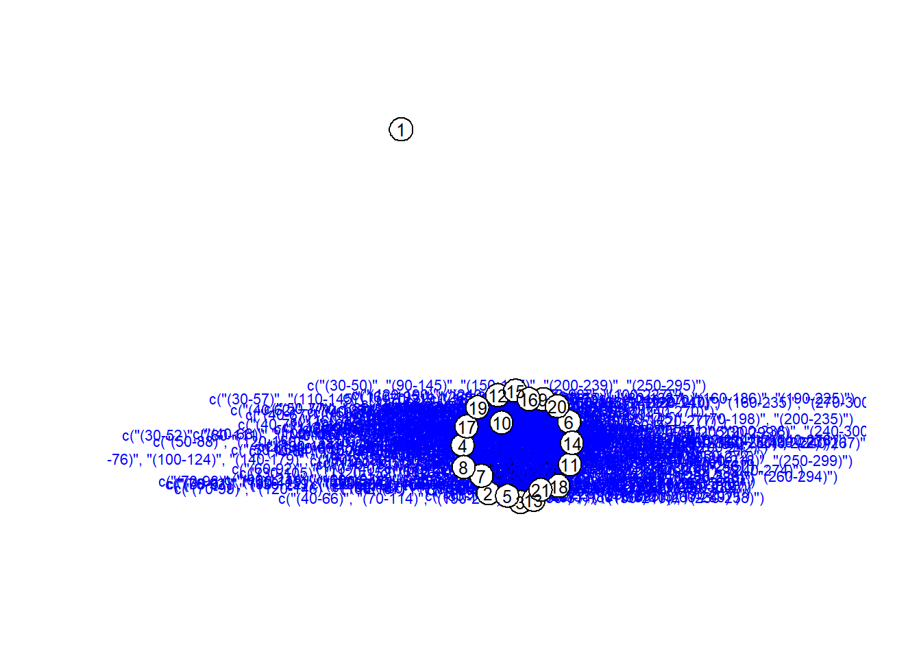
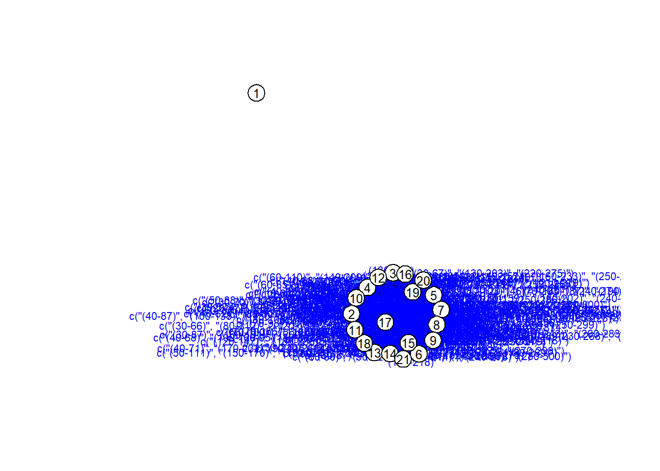
# Visualize the Temporal Network# Realize that visualization is lame coords =plot(net_dyn,displaylabels=TRUE,label.cex =0.8,label.pos =5,vertex.col ='white',vertex.cex =3,edge.label =sapply(get.edge.activity(net_dyn),function(e){paste('(',e[,1],'-',e[,2],')',sep='') }),edge.label.col ='blue',edge.label.cex =0.7)
coord <-network.layout.fruchtermanreingold(network.extract(net_dyn, at =1), NULL)# Plot separate moments in time:par(mfrow =c(2, 2)) times =c(1, 100, 200, 300) titles =paste("Network at t =", times)invisible(lapply(seq_along(times), function(i) {plot(network.extract(net_dyn, at = times[i]),main = titles[i],displaylabels =TRUE,label.cex =0.6,label.pos =5,vertex.col ='white',vertex.cex =5,coord = coord) }))
# tdist: distance from t = origin for v to affect the i^{th} node# previous: The node that immediately preceeded landing on the i^{th} node# gsteps: The number of "graph" steps to get to the i^{th} nodeplot(v1path, coord = coord,displaylabels =TRUE)# Observing the number of connections as a function of timeplot(tEdgeFormation(net_dyn, time.interval =1))# Observing graph-based density as a function of time dynamicdensity =tSnaStats( net_dyn,snafun ="gden",start =1,end =300,time.interval =1,aggregate.dur =10 )plot(dynamicdensity)# Observing betweenness in the graph over time dynamicbtw =tSnaStats( net_dyn,snafun ="centralization",start =1,end =300,time.interval =1,aggregate.dur =10,FUN ="betweenness" )plot(dynamicbtw)
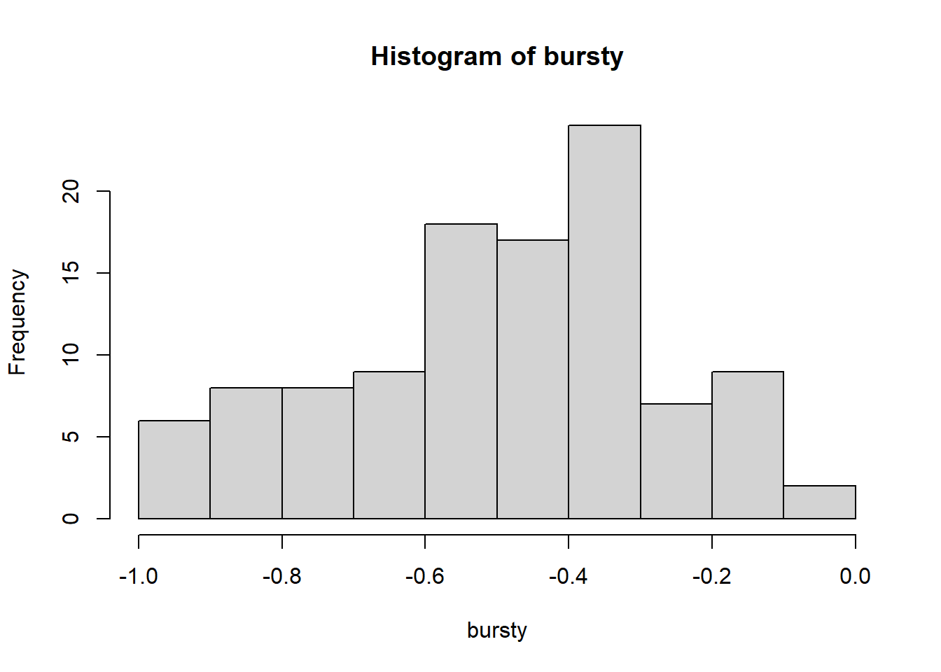
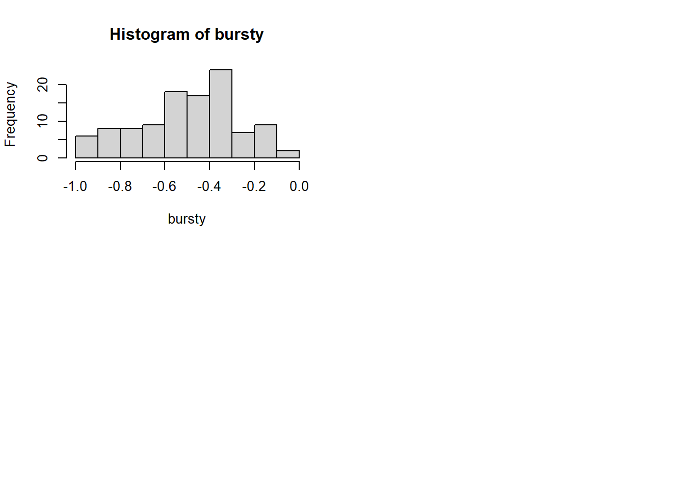
# Burstiness Burstiness =1# dense activity Burstiness =0#Poisson; "coin flip" Burstiness <0#Periodic; regularity in connections over time
Solution found! Final fit=31133.576 (started at 36424.759) (1 attempt(s): 1 valid, 0 errors)
Start values from best fit:
0.541509266466209
summary(ar1)$parameters
          name matrix row col  Estimate   Std.Error lbound ubound lboundMet
1 OUMod.A[1,1]      A   1   1 0.5415093 0.007444107     NA     NA     FALSE
  uboundMet
1     FALSE
# Can compare to different AR: osc$A$values =-0.60 sim.data =mxGenerateData(osc, nrows =1000)plot(x = (1:nrow(sim.data)), y = sim.data$AR1, type ="l",main ="Time-Series of AR1", ylab ="Values", xlab ="Time")
          name matrix row col    Estimate  Std.Error lbound ubound lboundMet
1 OUMod.A[1,1]      A   1   1  0.62172063 0.02297997     NA     NA     FALSE
2 OUMod.A[2,1]      A   2   1 -0.02204315 0.02297805     NA     NA     FALSE
3 OUMod.A[3,1]      A   3   1 -0.02635277 0.02298027     NA     NA     FALSE
4 OUMod.A[1,2]      A   1   2  0.01285982 0.02451216     NA     NA     FALSE
5 OUMod.A[2,2]      A   2   2  0.62969098 0.02451329     NA     NA     FALSE
6 OUMod.A[3,2]      A   3   2 -0.24716247 0.02451310     NA     NA     FALSE
7 OUMod.A[1,3]      A   1   3  0.23113522 0.02350982     NA     NA     FALSE
8 OUMod.A[2,3]      A   2   3  0.01534630 0.02350965     NA     NA     FALSE
9 OUMod.A[3,3]      A   3   3  0.62193553 0.02351152     NA     NA     FALSE
  uboundMet
1     FALSE
2     FALSE
3     FALSE
4     FALSE
5     FALSE
6     FALSE
7     FALSE
8     FALSE
9     FALSE