A static network is as a graph constructed from an edge list, where nodes represent entities and edges represent relationships between them.
Static networks are represented as \[G(V,E)\] where V is the set of nodes and E is the set of edges connecting those nodes. G=(V,E),the structure of the network is entirely defined by which nodes exist and which pairs of nodes are connected.
What are their shortcomings? I’m so glad you asked.
All interactions are aggregated over time into a single adjacency structure.
They compress all temporal information into a single snapshot. Information about when interactions occurred is lost. Static networks remove information about the ordering of events. This can lead to incorrect interpretations of paths, because the model treats all edges as if they exist simultaneously. Static networks cannot distinguish between different temporal sequences of interactions.
What information gets compressed and what does that compression imply?
When we convert a temporal system into a static network, we are compressing all information about time into a single aggregated structure. We lose the ordering, the timing, and the duration of interactions.
Not knowing the temporal sequencing of events can result in erroneous directional interpretations
i.e., A -> B at T = 1 and B -> C at T = 2
Thus, A can reach C but C cannot reach A
If we flatten a temporal graph/network then we lose that information
i.e., A -> B at T = 2 and B -> C at T = 1
Element of Time
Time is an important consideration is many types of networks.
Disease Spreading and Epidemiology
Air Transport and Logistics
Neuroscience and Brain Connectivity
Social Interactions
These networks would lose vital information without the consideration of time. Looking at a static network can distort centrality and connectivity measures, since nodes that are only briefly or sporadically connected may appear as permanently connected in a snapshot.
If we visualize the temporal network with edges as durations we see that…..
library(sna)
Loading required package: statnet.common
Attaching package: 'statnet.common'
The following objects are masked from 'package:base':

    attr, order
Loading required package: network
'network' 1.19.0 (2024-12-08), part of the Statnet Project
* 'news(package="network")' for changes since last version
* 'citation("network")' for citation information
* 'https://statnet.org' for help, support, and other information
sna: Tools for Social Network Analysis
Version 2.8 created on 2024-09-07.
copyright (c) 2005, Carter T. Butts, University of California-Irvine
 For citation information, type citation("sna").
 Type help(package="sna") to get started.
library(tsna)
Loading required package: networkDynamic
'networkDynamic' 0.11.5 (2024-11-21), part of the Statnet Project
* 'news(package="networkDynamic")' for changes since last version
* 'citation("networkDynamic")' for citation information
* 'https://statnet.org' for help, support, and other information
library(ndtv)
Loading required package: animation
'ndtv' 0.13.4 (2024-06-30), part of the Statnet Project
* 'news(package="ndtv")' for changes since last version
* 'citation("ndtv")' for citation information
* 'https://statnet.org' for help, support, and other information
# A dataframe is read in or loaded: df =read.csv("./df.csv") n_nodes =max(c(df$tail, df$head)) base_net =network.initialize(n_nodes, directed =FALSE)# The dataframe should be turned into a Temporal Network: net_dyn =networkDynamic(base.net = base_net,edge.spells = df[, c("onset", "terminus", "tail", "head")] )
Created net.obs.period to describe network
 Network observation period info:
  Number of observation spells: 1
  Maximal time range observed: 10 until 300
  Temporal mode: continuous
  Time unit: unknown
  Suggested time increment: NA
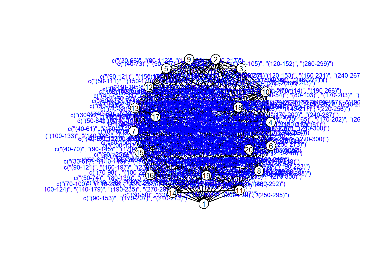
# Visualize the Temporal Network# Realize that visualization is lame coords =plot(net_dyn,displaylabels=TRUE,label.cex =0.8,label.pos =5,vertex.col ='white',vertex.cex =3,edge.label =sapply(get.edge.activity(net_dyn),function(e){paste('(',e[,1],'-',e[,2],')',sep='') }),edge.label.col ='blue',edge.label.cex =0.7 )
its a mess and lame.
Temporal Networks
An academic audience example: Conferences!
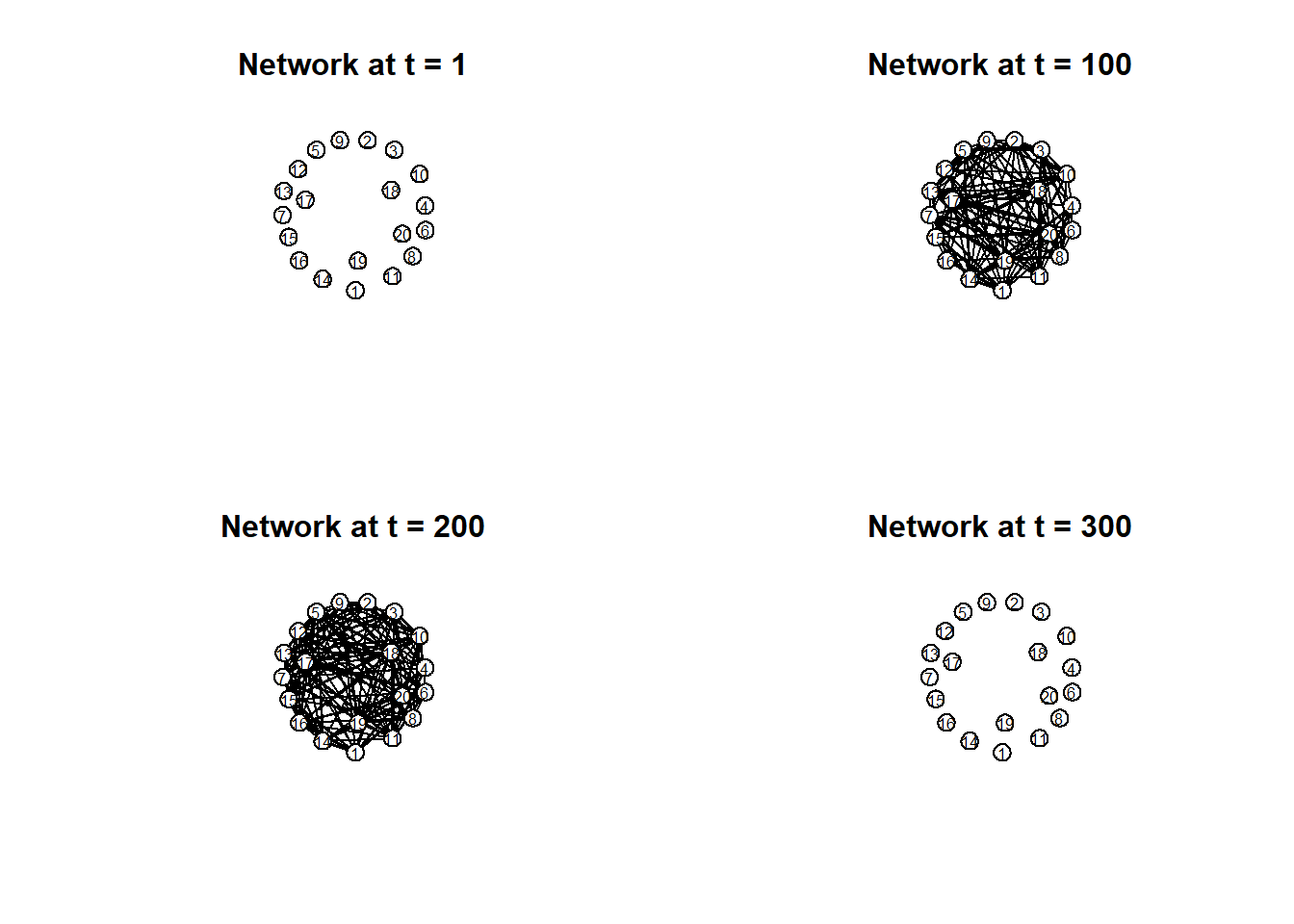
# Plot separate moments in time:par(mfrow =c(2, 2)) times =c(1, 100, 200, 300) titles =paste("Network at t =", times)invisible(lapply(seq_along(times), function(i) {plot(network.extract(net_dyn, at = times[i]),main = titles[i],displaylabels =TRUE,label.cex =0.6,label.pos =5,vertex.col ='white',vertex.cex =5,coord = coords ) }))
A bunch of smart maybe socially anxious people brought together for a weekend.
At t=1 everyone just arrived and is kind of awkward and not making much small talk. There is little connectivity.
At t=100 you run into your colleagues, people from grad school and what not, its less awkward, people are talking more, we see much more connectivity. You go to some talks and mill around.
At t=200 its maybe an evening poster session, people have drinks and are chatting alot. There is dense connectivity.
At t=300 weekend is over everyone is tired ready to go home and the connectivity decreases again.
Lets look at the math :’)
Lets redefine \[G(V, E)\] as the multilayer network, \[G(V, E, D)\]
We can extend the standard graph formulation G(V,E) into a multilayer representation G(V,E,D), where D represents another dimension, time
D represents a “dimension” of the network representing different layers
D corresponds to different layers of the network. Each layer can be interpreted as a separate slice of the system that captures a distinct context.
In temporal networks, layers are different slices of time
Each layer corresponds to a discrete time step or time interval, and the full network is then understood as a sequence of networks evolving across these layers.
So lets look at a more dynamic view of this conference network.
Calculating layout for network slice from time 1 to 11
Calculating layout for network slice from time 11 to 21
Calculating layout for network slice from time 21 to 31
Calculating layout for network slice from time 31 to 41
Calculating layout for network slice from time 41 to 51
Calculating layout for network slice from time 51 to 61
Calculating layout for network slice from time 61 to 71
Calculating layout for network slice from time 71 to 81
Calculating layout for network slice from time 81 to 91
Calculating layout for network slice from time 91 to 101
Calculating layout for network slice from time 101 to 111
Calculating layout for network slice from time 111 to 121
Calculating layout for network slice from time 121 to 131
Calculating layout for network slice from time 131 to 141
Calculating layout for network slice from time 141 to 151
Calculating layout for network slice from time 151 to 161
Calculating layout for network slice from time 161 to 171
Calculating layout for network slice from time 171 to 181
Calculating layout for network slice from time 181 to 191
Calculating layout for network slice from time 191 to 201
Calculating layout for network slice from time 201 to 211
Calculating layout for network slice from time 211 to 221
Calculating layout for network slice from time 221 to 231
Calculating layout for network slice from time 231 to 241
Calculating layout for network slice from time 241 to 251
Calculating layout for network slice from time 251 to 261
Calculating layout for network slice from time 261 to 271
Calculating layout for network slice from time 271 to 281
Calculating layout for network slice from time 281 to 291
Calculating layout for network slice from time 291 to 301
Calculating layout for network slice from time 301 to 311
render.d3movie( net_dyn,displaylabels =FALSE,# This slice function makes the labels workvertex.tooltip =function(slice) {paste("<b>Name:</b>", (slice %v%"name"),"<br>","<b>Region:</b>", (slice %v%"region") ) } )
caching 10 properties for slice 0
caching 10 properties for slice 1
caching 10 properties for slice 2
caching 10 properties for slice 3
caching 10 properties for slice 4
caching 10 properties for slice 5
caching 10 properties for slice 6
caching 10 properties for slice 7
caching 10 properties for slice 8
caching 10 properties for slice 9
caching 10 properties for slice 10
caching 10 properties for slice 11
caching 10 properties for slice 12
caching 10 properties for slice 13
caching 10 properties for slice 14
caching 10 properties for slice 15
caching 10 properties for slice 16
caching 10 properties for slice 17
caching 10 properties for slice 18
caching 10 properties for slice 19
caching 10 properties for slice 20
caching 10 properties for slice 21
caching 10 properties for slice 22
caching 10 properties for slice 23
caching 10 properties for slice 24
caching 10 properties for slice 25
caching 10 properties for slice 26
caching 10 properties for slice 27
caching 10 properties for slice 28
caching 10 properties for slice 29
caching 10 properties for slice 30
wrote animation HTML file to C:\Users\imjpark\AppData\Local\Temp\RtmpojyIr9\filef27c4a00eee.html
browser launching disabled because R is not in interactive mode
Modeling Network Metrics through Time
Pan and Saramäki define temporal closeness centrality using the following equation….
t(ij) = the average temporal distance (the average time it takes to reach node j from node i along the fastest time-ordered paths)
Temporal closeness centrality quantifies how quickly a node can reach all other nodes in a system by accounting for the specific timing and order of interactions.
How does it differ from “static” closeness?
Static distance in undirected networks is symmetric. Temporal distances are inherently non-symmetric, even if edges are undirected, the time-ordering of events means the fastest path from i to j may be much shorter than the path from j to i.
Reachability
In temporal networks, reachability defines which nodes can communicate with or influence others based on the timing and order of interactions. In static networks connectivity is whether a path exists, reachability in temporal systems is governed by time-respecting paths—sequences of contacts with non-decreasing times.
Contrast from a simple di-graph
They differ in how they handle transitivity.
Transitivity in Di-graphs: if a directed edge exists from A→B and another from B→C, then A is automatically connected to C via B.
Intransitivity in Temporal Networks: A can only reach C via B if the contact (A,B) occurs before or at the same time as the contact (B,C). If (B,C) happens at t=1 and (A,B) happens at t=20, the path is broken.
Dynamic Networks
In contrast to the temporal network, a dynamic network–for this class–is considered some form of model fitted to time-series observations.
temporal networks focus on when things happen, dynamic networks use the resulting parameters of a fitted model to define the edges of the network.
The parameters of the resulting fitted model form a dynamic network
What are some popular dynamic network “models”
Vector Autoregression (VAR):s a model for quantifying lagged associations between variables across time. A lag is a backward shift in time, with a lag of 1 denoting time t - 1.
Structural VAR (sVAR): An extension that accounts for contemporaneous relations (interactions occurring faster than the sampling rate) in a p-variate time-series.
Graphical VAR (gVAR): A model that produces non-directional contemporaneous networks of partial correlations based on the residual process noise of a VAR.
The Vector Autoregression (VAR)
\[\mathbf{\eta_{t}} = \mathbf{\Phi}\eta_{t-1} + \mathbf{\zeta}_{t}\] where \(\mathbf{\eta}\) represents a \(p\)-variate vector of scores on our latent variables, \(\mathbf{\Phi}\) represents our \(p\times p\) regression coefficients matrix relating past scores on our latent variables with current scores, and \(\mathbf{\zeta}\) is our \(p\)-variate vector of residuals \(\{\mathbf{\zeta}\} \sim \text{WN}(0, \mathbf{\Psi})\) and \(\mathbf{\Psi}\) is the \(p\times p\) matrix of innovation covariances.
Instead of modeling one outcome, VAR treats all variables as jointly evolving, where each variable is predicted by its own past and the past of the others.
Each variable at time t is a weighted combination of past values.
The weights (in Φ) tell you how much a variable influences itself over time (autocorrelation) and how much it influences other variables over time (cross-lagged effects)
example: Does low sleep yesterday → higher stress today?
Basically asks how do multiple variables predict each other over time?
GVAR models non-directional associations on the residual process noise of a VAR, which is a gaussian graphical model. These models utilize the inverse of the sample covariance matrix to estimate conditional associations between variables.
It creates non-directional contemporaneous networks of partial correlations.
Asks which variables are conditionally dependent at the same time, after removing lagged effects?
The SVAR
Slightly different model notation:
\[\mathbf{\eta_{t}} = \mathbf{A}\eta_{t} + \mathbf{\Phi}^{*}\eta_{t-1} + \mathbf{\zeta}_{t}^{*}\] where \(\mathbf{A}\) represents a \(p\times p\) matrix of contemporaneous effects with \(0\)’s along the diagonal, \(\mathbf{\Phi}^{*}\) is the \(p\times p\) matrix of lagged effects, and \(\mathbf{\zeta}^{*}\) is the \(p\)-variate vector of residuals assumed normally distributed with an identity covariance, \(\{\mathbf{\zeta}^{*}\} \sim \text{WN}(0, \mathbf{I}_{p})\).
SVAR models instantaneous directional effects.
SVAR adds an additional p x p matrix of contemporaneous effects, A, at time, t to the VAR and the asterisk has been dropped from Φ to differentiate it from the VAR, Φ*, coefficient matrix.
Asks which variables directly influence others immediately, within the same time step?
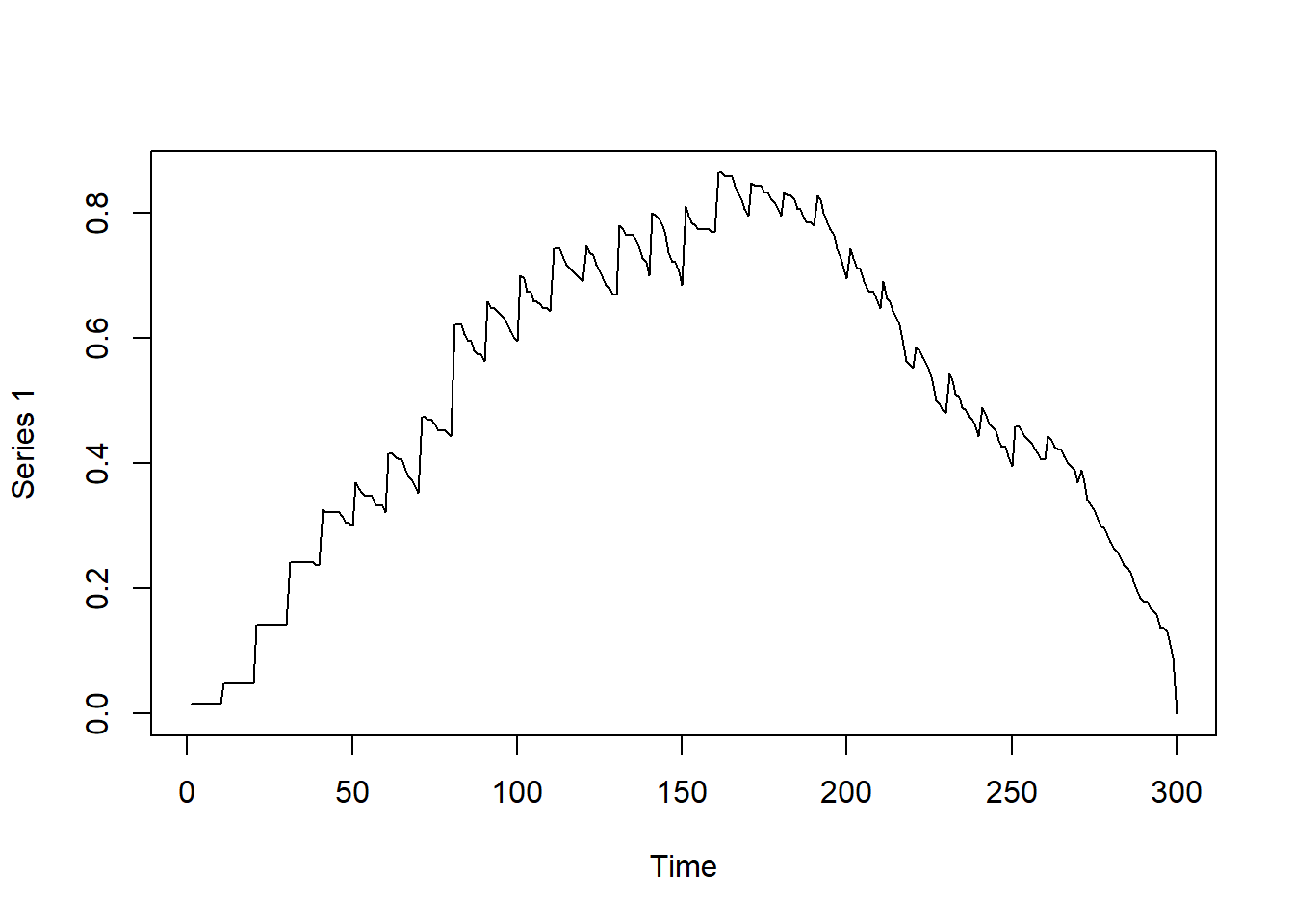
library(sna)library(OpenMx)library(tsna)library(ndtv)library(qgraph)###---###---###---###-### Preparing Data ######---###---###---###-# df = read.csv("C://Users/imjpark/Desktop/stn.csv")# df$tail = df$tail + 1# df$head = df$head + 1# df$min_node = pmin(df$tail, df$head)# df$max_node = pmax(df$tail, df$head)# df$tail = df$min_node# df$head = df$max_node# df$min_node = NULL# df$max_node = NULL# df_unique = df[!duplicated(df[, c("onset", "terminus", "tail", "head")]), ]###---###---###---###-### Tutorial Goals ######---###---###---###-## Graduate - 290# My hope is that you'll use this code to demonstrate mastery over the content and explain# Empirically and analytically, what these functions do and their limitations# Your use of this code can be empirically-based or acknowledge the simualted nature of# The data to push the boundaries of these approaches# You may use the code in whatever way you want; please try to hone in on identifying# Times when methods may be more or less appropriate for a given research quesiton# And what those research questions may be in various fields# Look at Forward Influence of the v^{th} node#v1path = tPath(net_dyn, v = 1, direction = "fwd")#print(v1path)# tdist: distance from t = origin for v to affect the i^{th} node# previous: The node that immediately preceeded landing on the i^{th} node# gsteps: The number of "graph" steps to get to the i^{th} node#plot(v1path, # coord = coords,# displaylabels=TRUE)# Plotting function from tutorial website:# plotPaths(# net_dyn,# v1path,# displaylabels = FALSE,# vertex.col = "white"# )# Observing the number of connections as a function of time#plot(tEdgeFormation(net_dyn, time.interval = 1))# Observing graph-based density as a function of time dynamicdensity =tSnaStats( net_dyn,snafun ="gden",start =1,end =300,time.interval =1,aggregate.dur =10 )plot(dynamicdensity)
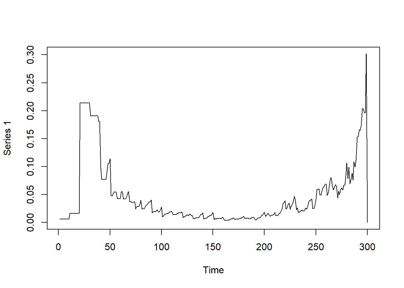
# Observing betweenness in the graph over time dynamicbtw =tSnaStats( net_dyn,snafun ="centralization",start =1,end =300,time.interval =1,aggregate.dur =10,FUN ="betweenness" )plot(dynamicbtw)
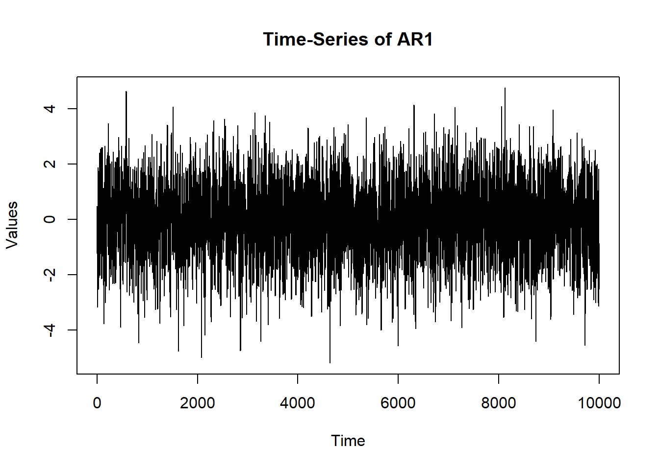
Solution found! Final fit=28308.549 (started at 33912.53) (1 attempt(s): 1 valid, 0 errors)
Start values from best fit:
0.600628831642041
summary(ar1)$parameters
          name matrix row col  Estimate   Std.Error lbound ubound lboundMet
1 OUMod.A[1,1]      A   1   1 0.6006288 0.008023318     NA     NA     FALSE
  uboundMet
1     FALSE
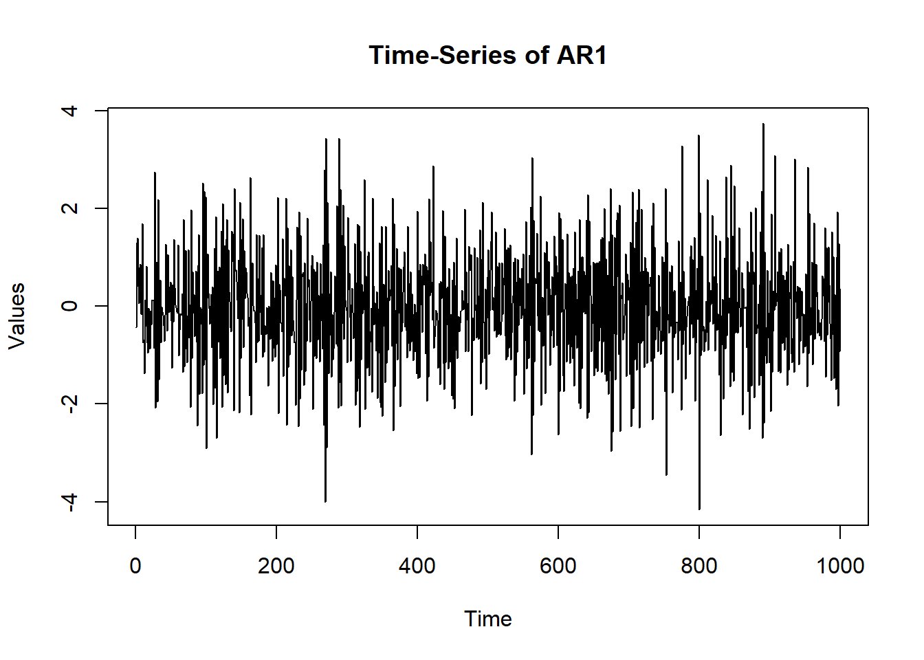
# Can compare to different AR: osc$A$values =-0.60 sim.data =mxGenerateData(osc, nrows =1000)plot(x = (1:nrow(sim.data)), y = sim.data$AR1, type ="l",main ="Time-Series of AR1", ylab ="Values", xlab ="Time")
name matrix row col Estimate Std.Error lbound ubound lboundMet
1 OUMod.A[1,1] A 1 1 0.607633136 0.02352499 NA NA FALSE
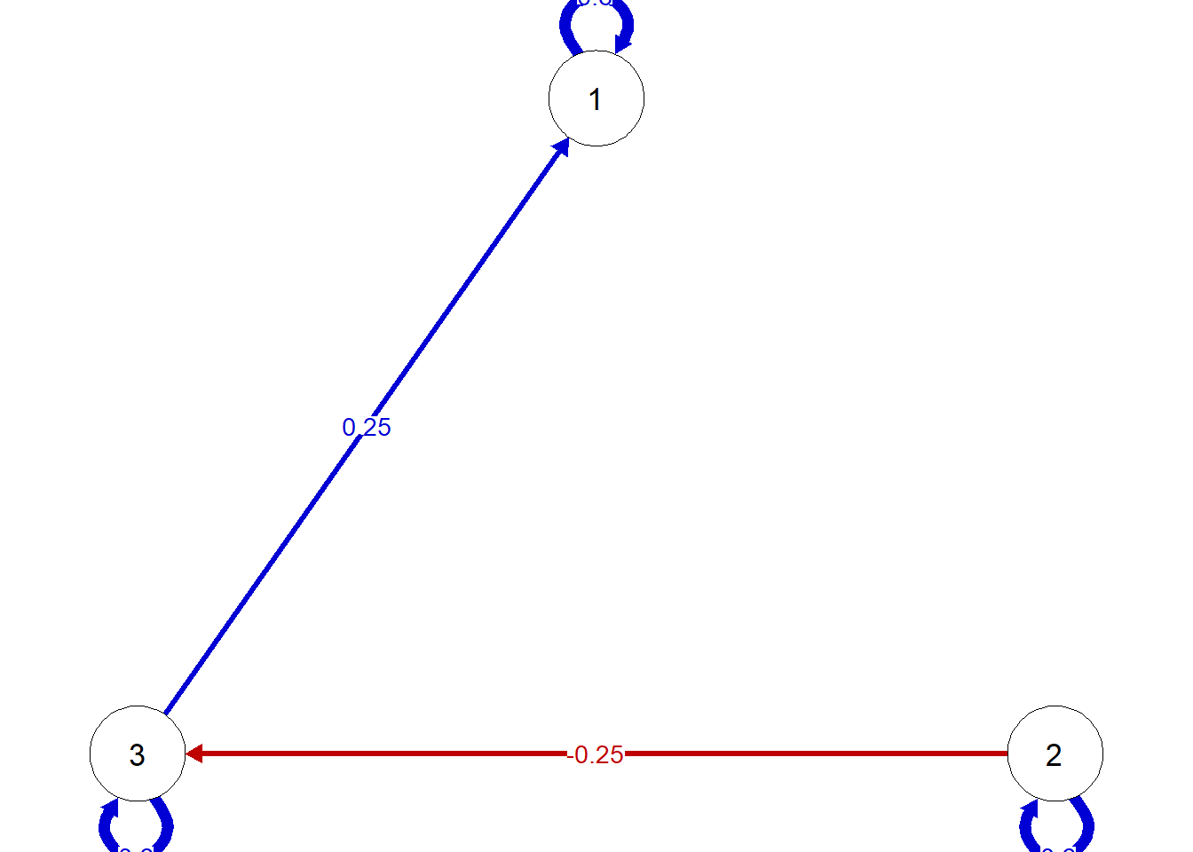
2 OUMod.A[2,1] A 2 1 -0.003594672 0.02352538 NA NA FALSE
3 OUMod.A[3,1] A 3 1 -0.031638774 0.02352654 NA NA FALSE
4 OUMod.A[1,2] A 1 2 0.001660937 0.02647742 NA NA FALSE
5 OUMod.A[2,2] A 2 2 0.590747377 0.02647791 NA NA FALSE
6 OUMod.A[3,2] A 3 2 -0.219879281 0.02648033 NA NA FALSE
7 OUMod.A[1,3] A 1 3 0.217771401 0.02535975 NA NA FALSE
8 OUMod.A[2,3] A 2 3 0.020462395 0.02536157 NA NA FALSE
9 OUMod.A[3,3] A 3 3 0.581282978 0.02536239 NA NA FALSE
uboundMet
1 FALSE
2 FALSE
3 FALSE
4 FALSE
5 FALSE
6 FALSE
7 FALSE
8 FALSE
9 FALSE