Multilayer and Multiplex Networks in Psychological Science
1. Simple Graphs
A simple graph is defined by:
\[G = (V, E)\]
In psychological networks, nodes might be symptoms, emotions, behaviors, questionnaire items, people, words, or brain regions. Edges might represent associations, temporal predictions, social interactions, similarity, or some other relationship defined by the study.
A common node-level measure is degree, the number of edges connected to a node. For a binary undirected graph, the degree of node \(i\) is:
\[k_{i} = \sum_{j \in V} a_{ij}\] where \({a_{ij} \in \{{0, 1}\}}\) represents the absence or presence of an edge between nodes \(i\) and \(j\) in the adjacency matrix \(A\).
The important point is simple: a single graph gives one view of a system but many real-world systems are often much more complicated than the structures we’ve discussed so far.
Let’s think about a single-layer network representation of grief, where each node represents experiences after hearing the news (praying, seek support, shock, sad, guilt, relief, cry, self-isolate, attend funeral, offer help, etc.), and the edges represent relationships between them (e.g. partial correlations). It can provide a summary of associations among grief-related experiences. But we also won’t know relationships between emotion (like sad, guilt) and behaviors (like attend funeral, seek support) as time goes by.
2. Why Add Layers?
Many psychological systems are not captured well by one network. The same nodes may be related differently depending on measurement mode, time, context, or relationship type.
For example, symptoms could be connected through:
- self-report responses,
- behavioral tasks,
- clinician ratings,
- physiological measurements.
A single graph would collapse these into one structure. A layered approach keeps them as separate.
A multilayer network introduces a layer dimension, allowing nodes and edges to be organized across multiple layers: each layer is a single netwrok that models an aspect in the complex system. It considers intra-layer (within layer) and inter-layer (between layers) connections among nodes. Together, we can better understand the structure and dynamics of the system.
In the most general case, a node in one layer can connect to any node in another layer. This broader framework includes temporal networks (Shout out to 🙌 Ella Rogers in 290 and Nicole and Keira in 190 👏), multiplex networks, and networks of networks (Boccaletti et al., 2014; Aleta & Moreno, 2018).
Outside of psychology, an example of multilayer networks is the transportation network for California: the nodes represent locations such as cities (e.g. Los Angeles, San Francisco, Sacramento), the edges represent the within layer connections between nodes in terms of the routes of travel (e.g. bus route, highways), and the layers represent the between layer connections depending on the modes of travel (e.g. public transit, driving, flights).
3. Multilayer, Multiplex, and Temporal Networks
Multilayer network
A multilayer network is the broadest category. Layers may represent different times, contexts, measurement systems, groups, levels of organization, or relationship types.
A multilayer network can be written as:
\[M = (G, C)\]
where \(G\) is the family of layer-specific graphs and \(C\) is the set of connections between layers.
Using the friendship network as an example with \(G = (V, E, D)\) graph formulation:
\(V\) represents nodes in every layer: you and other people that you know
\(E\) represents edges within-layer: who befriend/follow whom
\(D\) represents layers in terms of different social media platforms
A concrete way to think about this is as a block matrix. If we have \(L\) layers, the full layered network can be represented as a supra-adjacency matrix:
\[\mathcal{A} = \begin{pmatrix} A^{(1)} & C^{(12)} & \cdots & C^{(1L)} \\ C^{(21)} & A^{(2)} & \cdots & C^{(2L)} \\ \vdots & \vdots & \ddots & \vdots \\ C^{(L1)} & C^{(L2)} & \cdots & A^{(L)} \end{pmatrix}\]
The diagonal blocks, such as \(A^{(1)}\) and \(A^{(2)}\), are the adjacency matrices for the separate layers. The off-diagonal blocks, such as \(C^{(12)}\), represent connections between layers.
Supra-adjacency matrices are central for spectral analyses, diffusion, random walks, and other dynamics on multilayer networks (Boccaletti et al., 2014; Aleta & Moreno, 2018; Guo et al., 2016).
Multiplex network
A multiplex network is a special type of multilayer network. In a strict multiplex network:
- The same nodes appear in every layer.
- Interlayer connections only connect a node to its own replica in another layer.
Multiplex networks are often useful when the same units are connected by different relationship types.
Using the friendship network example again:
\(V\) represents nodes in every layer: you and other people that you know
\(E\) represents edges within-layer: who befriend/follow whom
\(D\) represents layers in terms of different social media platforms
Then each layer (e.g. facebook \(f\), instagram \(i\), linkedin \(l\)) consists of:
\(G_{f} = (V, E_{f})\) with \(E_{f} = \{(V_{1}, V_{3}), (V_{2}, V_{3})\}\)
\(G_{i} = (V, E_{i})\) with \(E_{i} = \{(V_{1}, V_{3})\}\)
\(G_{l} = (V, E_{l})\) with \(E_{l} = \{(V_{1}, V_{2})\}\)
So now we can have:
A family of layer-specific graphs: \(G = \{G_{f}, G_{i}, G_{l}\}\)
The set of inter-layer connection: e.g \({(({V_{1},f), (V_{1},i), (V_{1}, l))} \in C}\)
If we collapse everything into one network, we simply conclude that everyone is friend with each other. But it is not necessarily true. Depending on the types of relationship we have with each other and sometimes the function of different platforms, we might follow someone on one platform but not on other platfoms: I follow my high school friends on facebook and instagram but not linkedin, I follow my lab mates on instagram and linkedin but not facebook.
why that is informative).
Recap on Temporal Networks
As you may remember, temporal networks move beyond \(G = (V, E)\) (static) and extend into \(G = (V, E, D)\), where \(D\) represents layers in terms of different slices of time:
Each layer (time \(t\)) consists of a network: \(G_{t} = (V_{t}, E_{t})\)
A sequence of \(G_{t}\) is the family of layer-specific graphs: \(G = \{G_{1}, G_{2}, ... , G_{T}\}\)
Interlayer edges that link nodes across \(t\) is the set of connection between layers: \(C\)
In a way, we can bridge temporal network into the multilayer space by limiting the representation of layers as time. Yet, multilayer networks can have layers representing more than just time.
4. Simulate a Multiplex-Style Symptom Network
In this example, the nodes are symptoms and the layers are measurement modalities.
The simulated data are intentionally constructed so that each layer has a clear community pattern, but the community pattern changes across layers. This makes the community-detection section useful: the flattened graph will give each symptom only one community label, but the multilayer representation can show that a symptom can belong to different communities in different measurement contexts.
This is a multiplex because the layers describe different types of relationships among the same symptom set. We focus on intralayer edges and then add simple replica-to-replica coupling for the multilayer community detection section.
- Discussion/Brainstorm: how can we convert this multiplex network for symptoms into a more general multilayer framework? (I’ll go first )
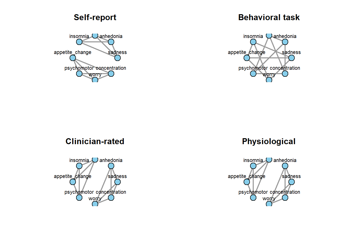
5. Plot the Individual Layers
The plotting code below uses the same circular layout for every layer. That way, when the edges change, you know the change is due to the layer and not due to a different layout algorithm.
Notice that the same symptoms do not group together in every layer. That is the point of the example.
6. Flatten the Multiplex Network
A multiplex network can be transformed into a flattened or aggregated network. Flattening means we collapse across layers.
In the table below:
fromandtoidentify a symptom pair;- each layer column says whether that edge appears in that layer;
weightcounts how many layers contain that edge.
              from            to self_report behavioral_task clinician_rated
1        anhedonia concentration           0               1               1
2        anhedonia       fatigue           1               1               0
3        anhedonia      insomnia           1               0               0
4        anhedonia   psychomotor           0               1               0
5        anhedonia       sadness           1               0               1
6        anhedonia         worry           0               0               1
7  appetite_change concentration           1               0               0
8  appetite_change       fatigue           0               0               1
9  appetite_change      insomnia           0               1               1
10 appetite_change   psychomotor           1               0               1
   physiological weight
1              1      3
2              0      2
3              0      1
4              0      1
5              1      3
6              1      2
7              0      1
8              1      2
9              1      3
10             1      3
If an edge has weight = 2, it appeared in two layers. If it has weight = 1, it appeared in only one layer.
7. Plot the Flattened Graph
Plotting the flattened graph is important. Otherwise, students only see the table and may not appreciate how much the graph changes after flattening.
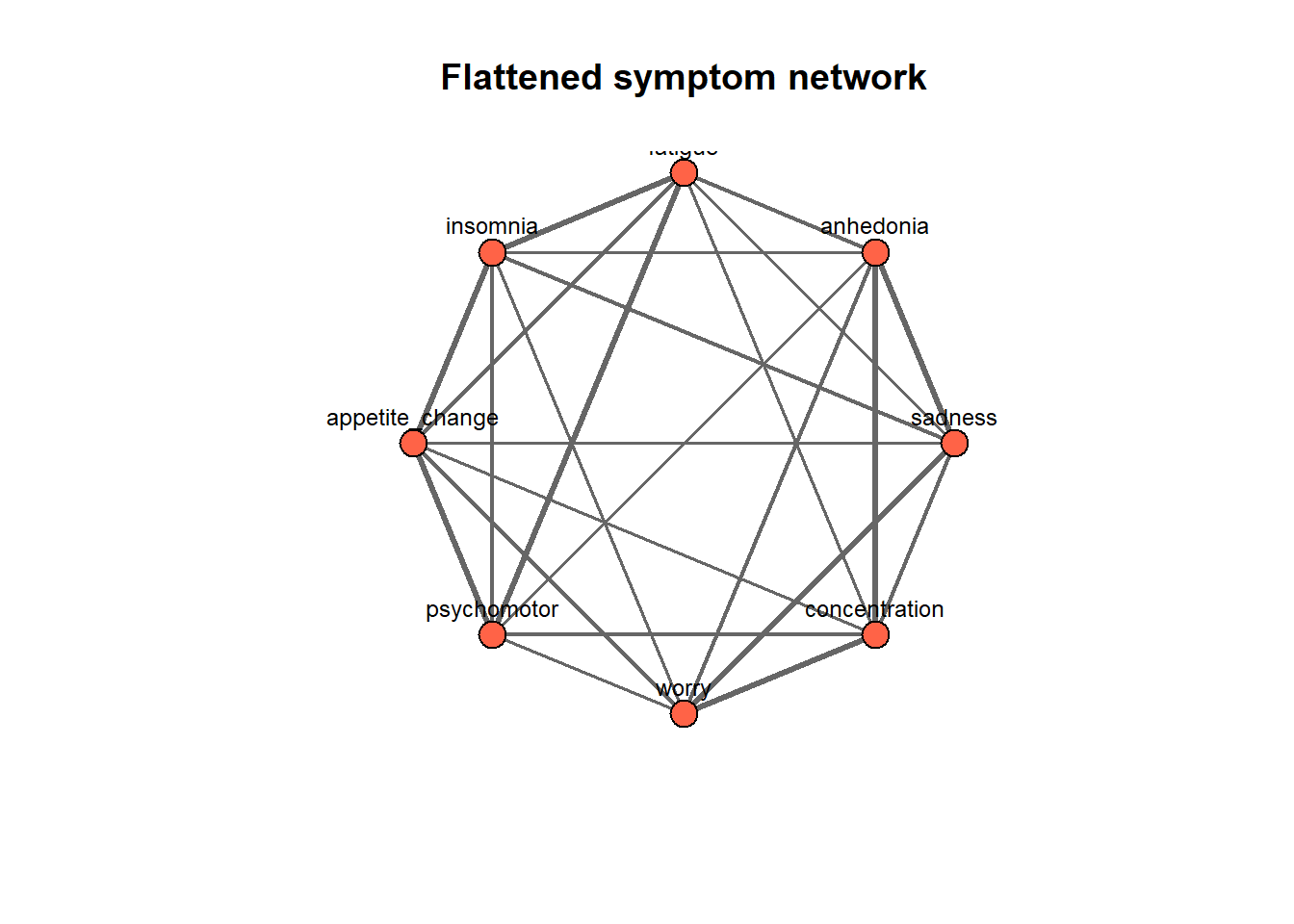
In this plot, thicker edges indicate symptom pairs that appear in more layers.
When we compare the flattened graph to the individual layer plots, the flattened graph is denser and less clearly tied to any one measurement modality.
8. What Is Lost When We Flatten?
In short, we can lose information when flattening a multilayer network into a single graph. For example, information about relationship type, context, measurement, time-varying, interactions, etc. is lost. These information can potentially masking important patterns and mechanisms underlying the system’s structure and dynamics.
9. Degree Within and Across Layers
In a single graph, degree is the number of edges attached to a node. In a multilayer network, degree can be computed separately for each layer.
For a multiplex network with \(L\) layers, the degree of node \(i\) can be represented as a vector:
\[\mathbf{k}_i = (k_i^{(1)}, k_i^{(2)}, \ldots, k_i^{(L)})\]
A simple summary is the total degree, or degree overlap:
\[o_i = \sum_{\alpha=1}^{L} k_i^{(\alpha)}\]
The vector is important because the same symptom can be highly connected in one layer and weakly connected in another. Reviews of multilayer networks emphasize that scalar summaries can miss layer-specific patterns, edge overlap, and cross-layer roles (Boccaletti et al., 2014; Aleta & Moreno, 2018).
When Low Degree Matters
A node with low degree in every layer can still matter, but the reason depends on the kind of layered graph.
In a multiplex network, the same nodes appear across layers. A node may have relatively few connections within each layer but it is one of the few nodes that always have connection in every layer. For example, in the friendship network from earlier, a low degree node can have no connection with other people but only connect with you across all social media platforms. This node can be the person that happen to be in the same high school, college, and work place as you.
In a multilayer network, interlayer edges can connect completely different types of nodes across layers. A node may have relatively few connections within each layer but it is bridge across layers. For example, in the infrastructure network from last week (a power grid layer connected to a communication router layer), a low degree node can serve a specific function to pass data between the two layers. If it fails, the layers become isolated from one another then lead to a cascading failure.
10. Community Detection on Multiple Layers
Community detection asks whether a network contains groups of nodes that are more densely connected internally than externally. In a single-layer graph, algorithms such as Louvain are often used to find communities by approximately maximizing modularity.
For multilayer networks, community detection is more interesting because the same symptom can have the same or different community memberships across layers.
Mucha et al. (2010) generalized modularity to multislice networks. In practice, packages such as multinet implement generalized Louvain-style methods using parameters such as \(\gamma\) for modularity resolution and \(\omega\) for interlayer coupling. The multinet documentation describes glouvain_ml(n, gamma = 1, omega = 1) and modularity_ml() for this purpose.
10.1 Build adjacency matrices
I (if pretending to be Jonathan) first implement a small base-R version using a supra-adjacency matrix. This is not meant to replace a polished package implementation. It is meant to make the idea visible and runnable.
10.2 Build The Supra-Adjacency
The functions then places layer adjacency matrices on the diagonal blocks and replica-to-replica coupling edges on the off-diagonal blocks. The coupling strength is \(\omega\).
                            sadness|self_report anhedonia|self_report
sadness|self_report                           0                     1
anhedonia|self_report                         1                     0
fatigue|self_report                           1                     1
insomnia|self_report                          1                     1
appetite_change|self_report                   0                     0
psychomotor|self_report                       0                     0
worry|self_report                             0                     0
concentration|self_report                     0                     0
                            fatigue|self_report insomnia|self_report
sadness|self_report                           1                    1
anhedonia|self_report                         1                    1
fatigue|self_report                           0                    1
insomnia|self_report                          1                    0
appetite_change|self_report                   0                    0
psychomotor|self_report                       0                    0
worry|self_report                             0                    0
concentration|self_report                     0                    0
                            appetite_change|self_report psychomotor|self_report
sadness|self_report                                   0                       0
anhedonia|self_report                                 0                       0
fatigue|self_report                                   0                       0
insomnia|self_report                                  0                       0
appetite_change|self_report                           0                       1
psychomotor|self_report                               1                       0
worry|self_report                                     1                       1
concentration|self_report                             1                       1
                            worry|self_report concentration|self_report
sadness|self_report                         0                         0
anhedonia|self_report                       0                         0
fatigue|self_report                         0                         0
insomnia|self_report                        0                         0
appetite_change|self_report                 1                         1
psychomotor|self_report                     1                         1
worry|self_report                           0                         1
concentration|self_report                   1                         0
The first block of the supra-adjacency matrix is the first layer. The later blocks contain the other layers. The off-diagonal values connect symptom replicas across layers.
10.4 Compare Flat Communities to Multilayer Communities
First, detect communities on the flattened graph.
  sadness
0.1666667
symptom flat_community
1 sadness 1
2 anhedonia 1
3 fatigue 2
4 insomnia 2
5 appetite_change 2
6 psychomotor 2
7 worry 1
8 concentration 1Now detect communities on the supra-adjacency matrix.
sadness|self_report
          0.7083333
state_node multilayer_community symptom
1 sadness|self_report 1 sadness
2 anhedonia|self_report 1 anhedonia
3 fatigue|self_report 1 fatigue
4 insomnia|self_report 1 insomnia
5 appetite_change|self_report 2 appetite_change
6 psychomotor|self_report 2 psychomotor
7 worry|self_report 2 worry
8 concentration|self_report 2 concentration
9 sadness|behavioral_task 4 sadness
10 anhedonia|behavioral_task 3 anhedonia
11 fatigue|behavioral_task 3 fatigue
12 insomnia|behavioral_task 4 insomnia
layer
1 self_report
2 self_report
3 self_report
4 self_report
5 self_report
6 self_report
7 self_report
8 self_report
9 behavioral_task
10 behavioral_task
11 behavioral_task
12 behavioral_taskPut the multilayer communities into a symptom-by-layer table.
          symptom self_report behavioral_task clinician_rated physiological
1         sadness           1               4               5             7
2       anhedonia           1               3               5             7
3         fatigue           1               3               6             8
4        insomnia           1               4               6             8
5 appetite_change           2               4               6             8
6     psychomotor           2               3               6             8
7           worry           2               4               5             7
8   concentration           2               3               5             7
10.5 Plot flat and multilayer community results
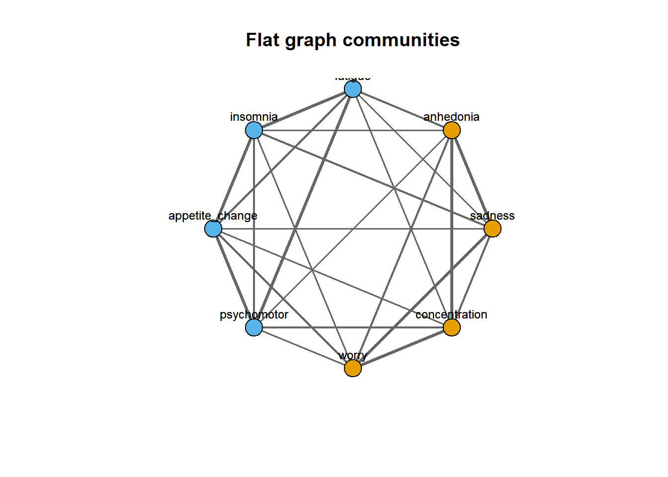
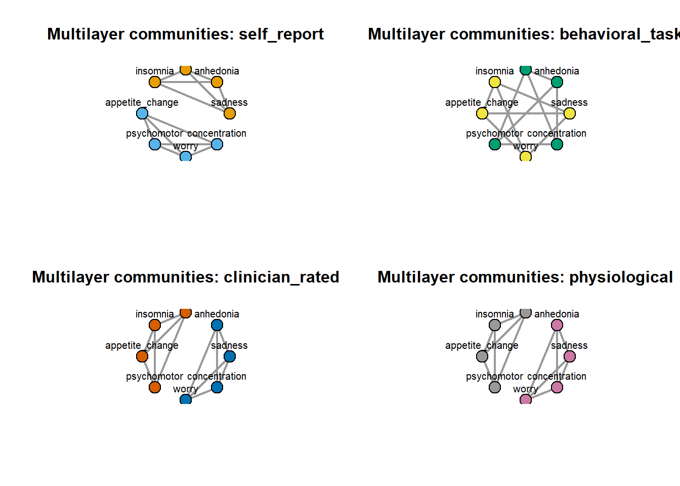
The flattened graph gives one partition of symptoms. The multilayer plot shows that the community structure depends on the measurement layer. This is why community detection should not stop at the flat graph.
11. Why This Matters in Psychological Science
A symptom can look different depending on the measurement layer. We can also be creative about what is the node, edge, and layer in the networks given our questions.
Some examples for brainstorming:
- Prolonged grief over time
- Cooperative behaviors across relationship types
- Personality inventory administrated in different languages
Multilayer networks matter in psychological science because we can model phenomena and processes as interconnected systems with a more realistic representation.
12. Caveats & Discussion Questions
Layers require theory
- Discussion question: if we don’t strong theory, how can we decide on our layers?
Interlayer edges require interpretation
- Discussion question: what measures (other than degree) can we adapt from single-layer network?
Flattening is sometimes useful:
- Discussion question: can less be more? do we always lose (meaningful) information when flatten?
Takeaways
A simple graph gives one view of a system. A multiplex or multilayer network lets us keep track of different views at the same time.
The supra-adjacency matrix is a useful way to see the whole layered system as one structured object: layer-specific adjacency matrices sit on the diagonal, and interlayer connections sit off the diagonal.
For psychological science, this matters because symptoms, behaviors, emotions, words, people, and brain regions may relate differently across measurement systems, contexts, or time. Flattening can be useful, but it should be treated as a modeling decision, not as a harmless default.