Cascading Failures
Failures (joke goes here)
What actually is a failure? In short, a failure is just a state of either a node or an edge! For example, we can imagine an node failing as a shutdown of a large power plant or the activation of a symptom. An edge failure could be something like a power line falling or removing the connection between a stimulus and fear response. The label failure is mostly arbitrary, but for the most part is applied to whatever state is the worse one out of two possible states.
Edge vs Vertex Failure
Like the decision to label one state a failure over the other, a focus on edge vs vertex failure is similarly context-dependent. Some situations are best modeled by edge failure, such as road or cable destruction in transport and information networks. Other situations might be best modeled by node failure, like analyzing the robustness of a city’s power generation grid.
What happens when they do fail?
In a cascading failures context, the failures chain (or perhaps even cascade) throughout the entire network. The central idea is that the state of one node (or edge) has some amount of influence on how likely its neighbors are to fail (or its failure threshold). For example, a non-failed node whose neighbors are 80% failures has a higher chance of also failing than a node whose neighbors are only 20% failures.
What are some real world networks and their failures?
There are some applications given already like power grids and transportation networks, but what would it mean for something like a psychological network to “fail”? Or what would it mean for a social network to fail?
Recap on Graph Structures
Time for a quick recap on graph structures! This is a very important determinant of the resilience of a network.
Erdős–Rényi(ER) Random Graphs
ER random graphs are the simplest of all graph structures, only needing a number of nodes and a probability of connection between two nodes to make one! This creates a very random graph, notably lacking a number of qualities that are often found in real-world applications like hubs and clusters
set.seed(14)
er <- sample_gnp(n=10, p=.5)
plot(er)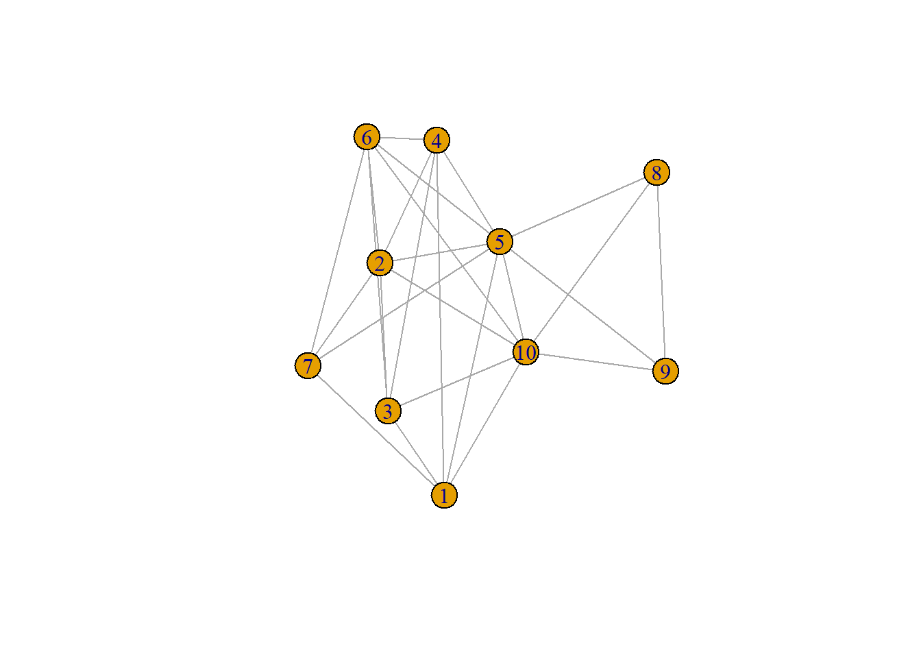
Barabási–Albert(BA) Random Graphs
BA random graphs are more interesting and often more useful as they aim to incorporate hubs, something that an ER random graphs can not do intentionally. BA graphs are sometimes labeled as “scale-free” graphs which means that the degree distribution of the graph follows a power law, being distributed as \(k^{-\gamma}\), where gamma is typically within 2-3.
But! This only describes a property of BA random graphs, so how are they actually made? BA random graphs are generated using Preferential Attachment, an algorithm which pretty much means that the graph is generated step-by-step and the nodes generated at each step prefer to link to the most popular node at the time. Step-by-step the algorithm is as follows:
Start with a few nodes that are fully connected and specify a number of links to be added to the graph at each time step
Generate a new node a however many links you specified in the beginning, these links have a higher probability of connecting to the “popular” nodes
Repeat step 2 until you have the number of nodes you want for your network
The probability of connection between the new node and the \(i^{th}\) node in the network is as follows: \[\Pi(i) = \frac{deg(i)}{\sum_{j}deg(j)}\]
g = sample_pa(n = 20, power = 1)
V(g)$name = as.character(1:vcount(g))
nodes = data.frame(id = V(g)$name, label = V(g)$name)
edges = igraph::as_data_frame(g, what = "edges")
visNetwork(nodes, edges) %>%
  visOptions(highlightNearest = TRUE, nodesIdSelection = TRUE) %>%
  visPhysics(stabilization = TRUE) %>%
  visInteraction(dragNodes = TRUE, dragView = TRUE)
bal <- list(
ba1 = sample_pa(n = 3, power = 1, m = 2, directed = F),
ba2 = sample_pa(n = 5, power = 1, m = 2, directed = F),
ba3 =sample_pa(n = 10, power = 1, m = 2, directed = F)
)
par(mfcol=c(1,3))
invisible(lapply(bal, plot, vertex.size = 25))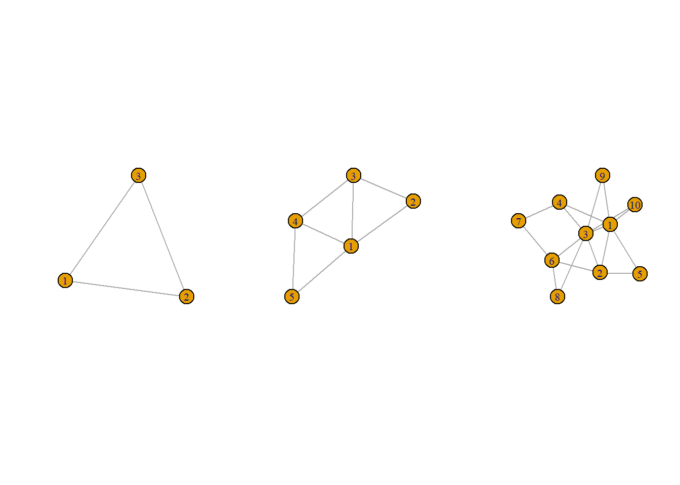
A Side Note on Assortative Mixing
Assortative mixing is another property of graph topology (or otherwise known as the shape of the graph) that describes the way nodes with many connections connect to other nodes. If a node with many connections tend to connect to other many-connected nodes then the graph can be said to display assortative mixing. If it doesn’t and nodes with many connections tend to be connected to nodes with few connections then the graph can be said to display disassortative mixing.
mixing <- list(
  assmix <- sample_gnp(n=10, p=.7),
  nonmix <- make_graph(edges = c(1,6,
                                 1,2,
                                 1,3,
                                 1,4,
                                 1,5,
                                 6,7,
                                 6,8,
                                 6,9,
                                 6,10), n=10, directed = FALSE)
)
par(mfcol=c(1,2))
invisible(lapply(mixing, plot, layout = layout_with_fr))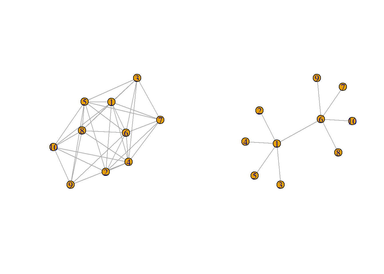
Watts-Strogats Small Worlds (WS or Small Worlds)
A small world graph, similarly to a BA random graph, aims to improve on ER random graphs by introducing some clustering and hubs. To create a small world graph, you only need to define number of nodes, average degree, and rewiring probability. What is the rewiring probability? Well the small world starts with a ring graph with the desired specifications which is then altered by the small world algorithm. The algorithm iterates over each node and (randomly) chooses another node and then, based on the provided probability, rewires the link to that one.
g = sample_smallworld(dim = 1, size = 20, nei = 2, p = .5)
V(g)$name = as.character(1:vcount(g))
nodes = data.frame(id = V(g)$name, label = V(g)$name)
edges = igraph::as_data_frame(g, what = "edges")
visNetwork(nodes, edges) %>%
  visOptions(highlightNearest = TRUE, nodesIdSelection = TRUE) %>%
  visPhysics(stabilization = TRUE) %>%
  visInteraction(dragNodes = TRUE, dragView = TRUE)
wss <- list(
ws1 <- sample_smallworld(dim=1, nei=2, size = 10, p=0),
ws2 <- sample_smallworld(dim=1, nei=2, size = 10, p=.1),
ws3 <- sample_smallworld(dim=1, nei=2, size = 10, p=.5)
)
par(mfcol=c(1,3))
invisible(lapply(wss, plot, layout= layout_in_circle))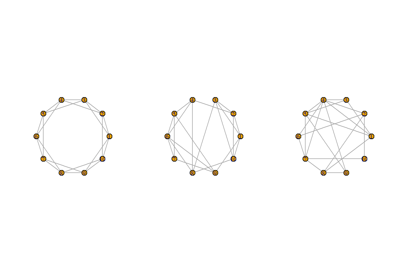
When do these different graph structures come up in real world applications?
The second two come up a lot! From electrical grids to transport networks to social circles, hubs and clustering appears literally everywhere in the real world. Random graphs are much more difficult to find, with random graphs often being used as a point of comparison for network studies.
How would these different structures hold up against failure?
Just a brief primer, but later on we’ll see that they all have different reactions to system shocks and differing resiliences to cascading failure!
But what is a cascading failure, exactly? (Watts Cascading Failure Model)
One possible model is outlined in Watts, 2002! Based around the idea of an information cascade in which a lot of people end up making similar decisions because they’re seeing the same decision being made by others around them. Based on this idea, Watts proposed a model for information cascade based on nodes’ individual thresholds and how many of its neighbors have already succumbed to failure. The model is as follows
- There is a starting network in which each node has their own personal threshold that will make them “fail” and all nodes start having not failed yet
- The network is perturbed or shocked by something and some nodes succumb to failure (perhaps some new product or shocking news)
- One node at random in the network checks their neighbors for failures and, if they have enough failures for neighbors to meet or exceed their failure threshold, they fail as well
- Repeat step 3 until there is no more spreading failure
Mathematically, it goes like this
- Define each node has \(k\) neighbors and a threshold fraction \(\phi\), with two possible states, 0 (normal) or 1 (failure)
- All nodes start in state 0
- \(\phi\) is the fraction of a node’s neighbors that must be in state 1 for the node to flip to state 1, all of which are taken from some distribution \(f(\phi)\) normalized such that \(\int^{1}_{0}f(\phi) = 1\)
- Construct graph with \(n\) nodes that have \(k\) neighbors with probability \(p_k\) and average neighbors \(z\), all nodes start in state 0
- In other words, a graph of \(n\) nodes, \(k\) degree distribution, and \(z\) average degree
- Shock your newly created graph by taking some small fraction of nodes \(\Phi_0 \ll 1\) and making switching them to state 1 (making them fail) at what is now time \(t=0\)
- Have one node calculate the fraction of its neighbors that are in state 1 (have failed) and compare against its threshold fraction \(\phi\), if it meets or exceeds its threshold, then fail
- Repeat step 3 until there’s no more change in the network
Now knowing how a cascade happens, how do you think the different graph structures will handle a cascade?
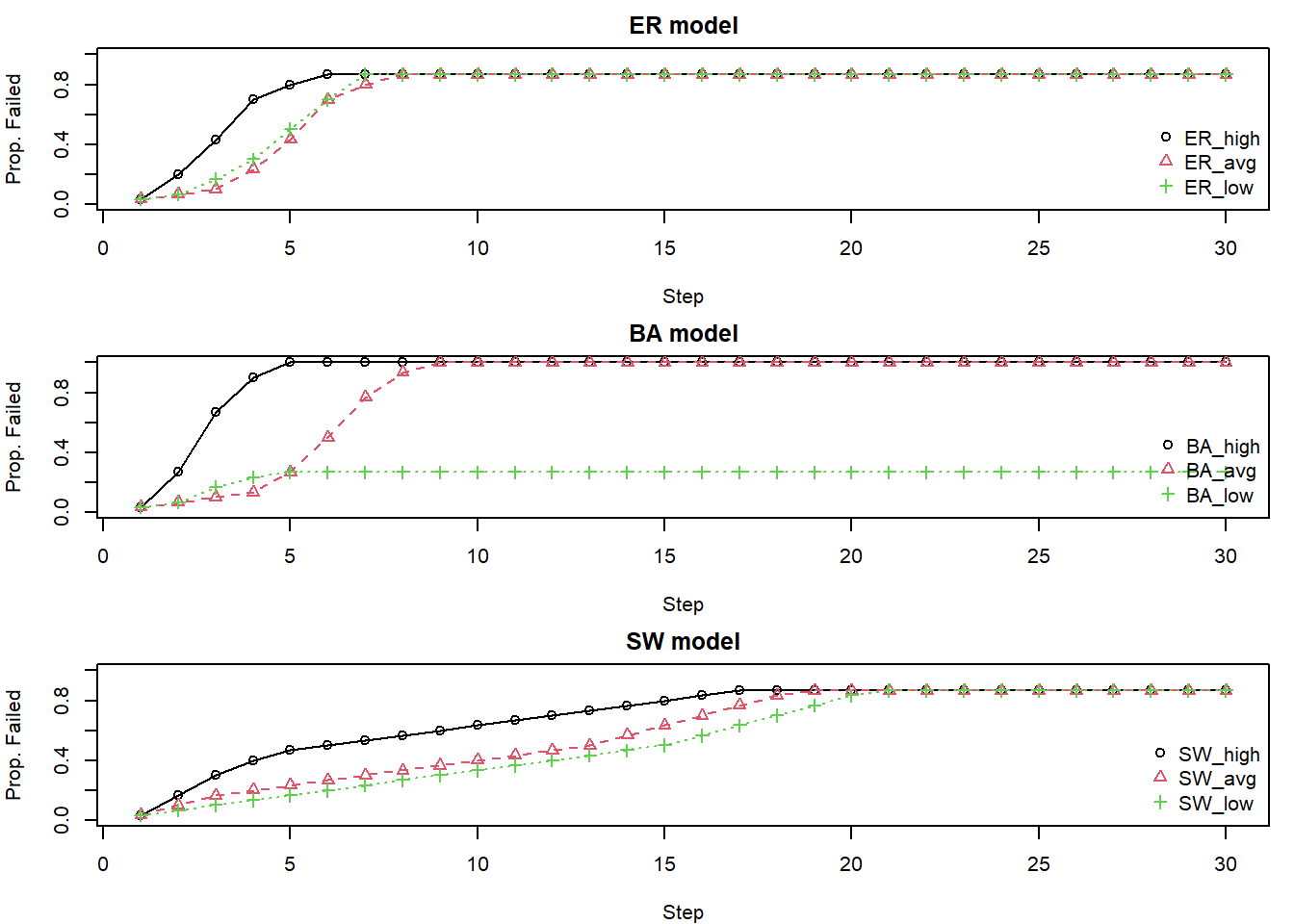
They all handle it differently! ER random graphs generally are quite vulnerable to failure across the board. Small worlds seem to fail slowly but always fail, but BA random graphs can, in some situations, resist complete network failure.
cascade.Watts = function(g, thrsh.lim = c(0.05, 0.90), max.steps = 10000){
  Cascades = list()
  metrics = igraph::degree(g)
  # Identify the high, average, and low degree vertices
  max_node = which.max(metrics)
  if(min(metrics, na.rm = TRUE) == 0){
    min_node = which.min(ifelse(metrics != 0 & !is.na(metrics), metrics, 999))
  }
  else(min_node = which.min(ifelse(!is.na(metrics), metrics, 999)))
  avg_node = sample(which(abs(metrics - floor(mean(metrics, na.rm = TRUE))) == min(abs(metrics - floor(mean(metrics, na.rm = TRUE))), na.rm = TRUE) & !is.na(metrics)), 1)
  seeds = list(high = max_node,
               avg = avg_node,
               low = min_node)
  # For the high, middle, and low vertices initiate a cascade
  for(name in names(seeds)) {
    target = seeds[[name]]
    if(thrsh.lim[1] > thrsh.lim[2]){
      message("First limit should be the lower limit! Flipping for you")
      thrsh.lim = c(thrsh.lim[2], thrsh.lim[1])
    }
    # Uniformly apply thresholds to all vertices between limits
    V(g)$threshold = runif(vcount(g), min = thrsh.lim[1], max = thrsh.lim[2])
    V(g)$state = 0
    V(g)$state[target] = 1
    flip.count = c(sum(V(g)$state))
    step = 0
    # Initiate Cascade
    while(step < max.steps) {
      step = step + 1
      new.state = V(g)$state
      # For each vertex, check if it failed. If so, skip
      # If not, then identify its neighbors
      # Check how many of the current vertex's neighbors have failed relative to total
      # Compare to threshold; if bigger then fail
      # Repeat
      for (v in V(g)) {
        if (V(g)$state[v] == 1) next
        neighbors.v = neighbors(g, v)
        if (length(neighbors.v) == 0) next
          active_fraction = sum(V(g)$state[neighbors.v]) / length(neighbors.v)
        if (active_fraction >= V(g)$threshold[v]) {
          new.state[v] = 1
        }
      }
      if(all(new.state == V(g)$state)) break
      V(g)$state = new.state
      flip.count = c(flip.count, sum(V(g)$state))
    }
    Cascades[[name]] = flip.count / vcount(g)
  }
  names(Cascades) = c("High", "Average", "Low")
  return(Cascades)
}

# Initial Parameters for Simulation
n_nodes = 30

# Simulation Function
sim.funk = function(rep_id) {
  set.seed(3887891 + rep_id)
  g_ba = sample_pa(n = n_nodes, power = 1, m = 1, directed = FALSE)
  g_er = sample_gnm(n = n_nodes, m = ecount(g_ba), directed = FALSE)
  g_sw = sample_smallworld(dim = 1, size = n_nodes, nei = floor(ecount(g_ba)/n_nodes), p = 0.05)
  ER.set = cascade.Watts(g_er, c(0.1, 0.20), 10000)
  BA.set = cascade.Watts(g_ba, c(0.1, 0.20), 10000)
  SW.set = cascade.Watts(g_sw, c(0.1, 0.20), 10000)
  list(
    ER_high = ER.set$High,
    ER_avg  = ER.set$Average,
    ER_low  = ER.set$Low,
    BA_high = BA.set$High,
    BA_avg  = BA.set$Average,
    BA_low  = BA.set$Low,
    SW_high = SW.set$High,
    SW_avg  = SW.set$Average,
    SW_low  = SW.set$Low
  )
}

results = sim.funk(1245)
models = c("ER","BA","SW")
max_len = 30
op = par(mfrow=c(3,1), mar=c(4,4,2,1))

for(m in models) {
  idx = grep(paste0("^", m, "_"), names(results))
  raw = results[idx]
  mat = sapply(raw, function(v) {
    L = length(v)
    if (L < max_len) {
      c(v, rep(v[L], max_len - L))
    } else {
      v[1:max_len]
    }
  })

  matplot(1:max_len, mat,
          type = "o", pch = 1:3,
          col = 1:3, xlab = "Step",
          ylab = "Prop. Failed",
          main = paste(m, "model"),
          xlim = c(1, max_len),
          ylim = c(0, 1))
  legend("bottomright", legend = names(results)[idx],
         col = 1:3, pch = 1:3, bty = "n")
}
Network Control vs Cascading Failures
Last week we briefly talked about the idea of network control, the idea that tweaking or changing some activation states of specific nodes can change the state of a node down a farther path into a more desirable state, but often with side effects along the way. Cascading failures is a tool with a similar purpose of seeking the outcome of changes in a network, although with much more wide reaching effects than network control. Where network control seeks to move the state of the network into a more favorable position, often times the goal of a cascading failure model is to simulate the worst possible outcome for a network to find its most important features. Importantly, a major difference of cascading failures vs network control is that cascading failures strongly emphasizes the role of network structure while network control emphasizes overall network states through binary rules.
CASCADE model for Cascading Failures
This is another model for cascading failures (A bit more complicated than the last one)! This model, instead of determining failure through some fraction threshold of failures for neighbors, uses the idea of load. A load is the amount of some “stuff” that moves through a network that each component can hold or move a certain amount of. In this model, each component has some initial load which is the amount of “stuff” in the component at the first time step, which is randomly assigned to each component according to the preset minimum and maximum initial load.
To actually simulate the failure, each component also has some threshold that, if the load exceeds, makes the component fail. Under the situation the component fails, the load that was contained within that component is then redistributed to its neighbors or immediate connections, possibly overloading those as well.
In this model, to start a cascade, the network gets some disturbance, which is just an additional load added to each component.
For example, a power network using the cascade model might have components’ initial load be between [10,20] gigawatts and a disturbance of 2 gigawatts is applied to each component in the network. In this scenario, its likely that those extra 2 gigawatts being added to a component’s initial load makes its total load go over its limit and overloads it, making it redistribute its load to its neighbors, which may make its neighbors fail and so on, resulting in a cascade.
So we can probably think of what the “stuff” would be in physical networks like power grids, but what about less tangible ones like a psychological network?
For psychological networks, we don’t really know! Depending on the context, we can have some ideas about what it might be, but even then we probably wouldn’t be able very tangible
Follow up question: Does it matter what the “stuff” is?
I don’t know!
Formally, CASCADE models are defined by selecting a graph with \(N\) vertices that each share a random load value. The minimum value of a given load is \(L^{\text{min}}\) and the maximum load is \(L^{\text{max}}\). For all \(N\) vertices, they are given an initial load, \(L_{j}\) which is distributed uniformly between \([L^{\text{min}}, L^{\text{max}}]\).
The normalized initial load for the \(j^{th}\) vertex is given by \(\ell_{j}\) where:
\[ \ell_{j} = \frac{L_{j} - L^{\text{min}}}{L^{\text{max}} - L^{\text{min}}}\] Under this normalization scheme, \(\ell_j\) is another random variable distributed uniformly on an interval of [0,1]
An edge or node of the graph fails when their load exceeds the node or edge’s \(L_{fail}\) value. When an edge or vertex does fail, it redistributes a fixed amount of load \(P\) to its neighbors. The amount of load transferred to neighbors can be expressed by the normalized load increment \(p\) given by \[p=\frac{P}{L^{max}-L^{min}}\].
A cascade is initiated using some initial disturbance \(D\) that adds additional load to each node and edge. This disturbance value can be expressed by a normalized disturbance value \(d\) given by \[d=\frac{D+L^{max}-L^{fail}}{L^{max}-L^{min}}\]
### "Complex" Xiang Cascade

cascade.Xiang = function(g, beta = 1, T = 1.2, alpha = 1, max.steps = 10000) {
  N = vcount(g)
  deg = igraph::degree(g)
  # Load is based on beta, alpha, and degree
  load0 = beta * (deg^alpha)
  cap = T * load0
  # Choose high, average, and lowest degree vertices
  high = which.max(deg)
  low = which.min(deg)
  avg = which.min(abs(deg - mean(deg)))[1]
  seeds = list(High=high, Average=avg, Low=low)
  results = lapply(seeds, function(seed) {
    load = load0
    failed = logical(N)
    # Kill the target
    # Find neighbors
    # Distribute failure to other neighbors
    # High degree neighbors take more load
    failed[seed] = TRUE
    nbrs = as.integer(neighbors(g,seed))
    if (length(nbrs)) {
      wts = deg[nbrs]^alpha
      load[nbrs] = load[nbrs] + load[seed]*(wts/sum(wts))
    }
    load[seed] = 0

    series = sum(failed)/N
    t = 1
    while (t < max.steps) {
      to_fail = which(!failed & (load > cap))
      if (!length(to_fail)) break
      for (v in to_fail) {
        failed[v] = TRUE
        nbrs2 = setdiff(as.integer(neighbors(g,v)), which(failed))
        if (length(nbrs2)) {
          w2 = deg[nbrs2]^alpha
          load[nbrs2] = load[nbrs2] + load[v]*(w2/sum(w2))
        }
        load[v] = 0
      }
      t = t+1
      series[t] = sum(failed)/N
    }
    series
  })

  names(results) = names(seeds)
  results
}


sim.funk = function(rep_id, n_nodes) {
  set.seed(15846 + rep_id)
  g_ba = sample_pa(n = n_nodes, power = 1, m = 2, directed = FALSE)
  g_er = sample_gnm(n = n_nodes, m = ecount(g_ba), directed = FALSE)
  g_sw = sample_smallworld(dim = 1, size = n_nodes, nei = floor(ecount(g_ba)/n_nodes), p = 0.05)
  ER.set = cascade.Xiang(g_er, beta = 1, T = 1.2, alpha = 1, max.steps = 1000)
  BA.set = cascade.Xiang(g_ba, beta = 1, T = 1.2, alpha = 1, max.steps = 1000)
  SW.set = cascade.Xiang(g_sw, beta = 1, T = 1.2, alpha = 1, max.steps = 1000)
  list(
    ER_high = ER.set$High,
    ER_avg  = ER.set$Average,
    ER_low  = ER.set$Low,
    BA_high = BA.set$High,
    BA_avg  = BA.set$Average,
    BA_low  = BA.set$Low,
    SW_high = SW.set$High,
    SW_avg  = SW.set$Average,
    SW_low  = SW.set$Low
  )
}
n_nodes = 30
results = sim.funk(34, n_nodes = n_nodes)
models = c("ER","BA","SW")
max_len = 30
op = par(mfrow=c(3,1), mar=c(4,4,2,1))

for(m in models) {
  idx = grep(paste0("^", m, "_"), names(results))
  raw = results[idx]
  mat = sapply(raw, function(v) {
    L = length(v)
    if (L < max_len) {
      c(v, rep(v[L], max_len - L))
    } else {
      v[1:max_len]
    }
  })

  matplot(1:max_len, mat,
          type = "o", pch = 1:3,
          col = 1:3, xlab = "Step",
          ylab = "Prop. Failed",
          main = paste(m, "model"),
          xlim = c(1, max_len),
          ylim = c(0, 1))
  legend("bottomright", legend = names(results)[idx],
         col = 1:3, pch = 1:3, bty = "n")
}
Watts’ Cascade vs CASCADE
We can already see that these models are aiming to do a very similar thing: model a cascade through a network. As such, they share a number of similar features like some threshold value and influence of one component on its immediate neighbors. Despite this, they achieve this goal in fairly different ways which can be broken down in a convenient bullet list:
Watts’ Cascade
- Only influence from neighbors existence
- Shock initiated by a small group of failures
- No edge failures
CASCADE
- Some “thing” moves through the network (uses Loads and Capacities)
- Shocks come from additional load added to components
- Can incorporate multiple components (nodes OR/AND edges)
These differences imply that the CASCADE model can model more complex relationships as it uses a more complex method of modelling failure requirements than just fraction of failed neighbors and it also can incorporate edge failures as well as node failures. (Although I think that it may suffer a little bit in interpretability)
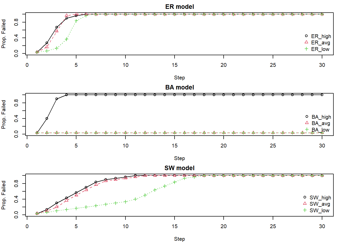
Also, as we have seen, these differences can see some noticeable differences in the performances of different graph structures.