Cascading Failures
Cascading Failures?
“One of the most dramatic processes that spread on complex networks is the cascade of failures when a failure in part of the system leads to further failures in the same and other systems which then continue to propagate. Eventually, the entire system could become dysfunctional and catastrophically collapse” (Valdez et al., 2020, p. 2).
Conceptually, a change in a network to one node could introduce subsequent changes in other nodes, potentially leading to whole system failure. Nodes in the system make binary decisions (on/off), and the decision is based on how neighbors connected to them behave — so-called binary decisions with externalities (Watts, 2002).
As cascading failures involve failures, I initially thought of something malignant and disastrous such as the pandemic we experienced, or a zombie apocalypse inspired by the cannibalism example we have enjoyed. However, cascading failures involve rather passive agents that do not seek out and actively attack a new host or a non-zombie human. Thus, better examples would be cultural fads, grassroots social movements, changes in social norms, and the diffusion of innovations in society (Watts, 2002). In the physical world, power and internet outages could serve as examples.
What are Failures in Graphs?
Do vertices fail? Do edges fail?
Edges and nodes can fail, meaning they could be removed. For nodes, think about power stations or cities that connect small towns. For edges, they may represent the roads connecting the city and the small towns, or cables that distribute electricity.
It is not hard to imagine that losing nodes could be more devastating than losing some dges. Also, in terms of recovery, replacing a cable may take fewer resources and less time than rebuilding a power station.
Or, let us take a lovelier example of beavers (from Dr. Park!): If beavers (nodes) leave some swamps because wolves hunt the entire beaver population, the whole ecological system would be disrupted since beavers manage critical ecological functions such as building dams — and being cute. To protect the beaver population, preventing wolves (nodes) from approaching beavers would likely save the whole ecological system.
What happens when they do fail?
Cascading failures leading to system collapse occur due to the dependencies within networks. Real-world examples of complex networks, such as infrastructure systems, are usually based on interdependent network structures where “the functionality of nodes in one network depends on the state of the nodes in other networks” (Valdez et al., 2020, p. 6).
We can then ask questions such as:
- Which nodes play the most important role in system failures?
- High-degree nodes (hubs) or low-degree nodes?
- How could we determine which nodes are more important than others?
- Through centrality measures?
In order to answer these questions, we should first discuss what kind of network structures we are looking at. By network structures, I mean the degree distributions of graphs, as different degree distributions have varying characteristics and assumptions. We should therefore first specify which distribution we are referring to.
Recap on Graph Structures
First things first! Degree is the number of connections a node has. In the context of cascading failures, we will discuss the load that nodes carry, as failures occur through the redistribution of loads — when redistributed load exceeds a node’s threshold or capacity, it triggers further system failures.
Erdős–Rényi Random Graphs
ER random graphs assume that the degree in a random graph follows a binomial distribution.
Just in case you get bored with all the letters so far:
the probability of a Vertex \(G(n, p)\) being linked to \(n-1\) other vertices is: \[ P(deg(v)= k)= \begin{pmatrix} n-1 \\ k \end{pmatrix}p^k(1-p)^{n-1-k} \] where \(k \in {0, 1, ..., (n-1)}\)
In the context of cascading failures, ER random graphs usually indicate homogeneous networks (with binomial and Poisson degree distributions). There are no nodes that have significantly more connections than others, and load distribution is pretty equal. Therefore, they are more resilient to random and load-based node failures (Kinney et al., 2005). This means that a single node failure may not lead to global impact, and the impact may stay local. Why? Because every node is pretty much the same — no single node really stands out in terms of load.
Let’s look at this demonstration:
ER animation
Watts-Strogatz Small-Worlds
While ER random graphs cannot accommodate the clustering aspects of complex networks, WS random graphs can! Starting from a regular lattice where every node connects to its \(k\) nearest neighbors, rewiring edges with probability \(\beta\) introduces shortcuts that create the small-world property while preserving local clustering.
WS random graphs are expressed as \(G_{WS}(n,k,\beta)\) where \(\beta\) is the probability of a node reassigning an edge.
WS animation
#|r echo = FALSE
g = sample_smallworld(dim = 1, size = 20, nei = 2, p = .5)
V(g)$name = as.character(1:vcount(g))
nodes = data.frame(id = V(g)$name, label = V(g)$name)
edges = as_data_frame(g, what = "edges")
visNetwork(nodes, edges) %>%
  visOptions(highlightNearest = TRUE, nodesIdSelection = TRUE) %>%
  visPhysics(stabilization = TRUE) %>%
  visInteraction(dragNodes = TRUE, dragView = TRUE)
Barabási–Albert Scale-Free Network
For investigating real-life complex networks, it might be better to assume heterogeneous networks. Barabási–Albert scale-free networks, where degree distribution follows a power-law distribution, can provide important insights.
\[ P(k) \sim k^{-\gamma} \] where \(2 < \gamma < 3\)
Here, the preferential attachment algorithm comes into play.
Preferential attachment means that when a new node enters a network, it is highly likely to connect to nodes that already have many connections. In this way, hubs increase their connections across a network as new nodes are introduced. Their connections and “influence” may grow as the network evolves and new nodes are incorporated following known procedures.
As you can see in the equation, the probability of a new node \(k^{th}\) getting connected to the \(i_{th}\) node depends on the relative strength of its connections compared to other nodes.
\[ \Pi(i) = \frac{deg(i)}{\Sigma_{j}deg(j)} \]
Assortativity is about whether highly connected nodes tend to connect to nodes similar to themselves. Networks exhibiting assortative mixing have high-degree nodes connecting to other high-degree nodes. Disassortative networks, on the other hand, have high-degree nodes connecting to those nodes with few connections (Ash & Newth, 2007).
As such, it is not hard to imagine that BA scale-free networks may be vulnerable to cascading failures due to their heterogeneity and the presence of hubs. Assortative networks would be particularly vulnerable since more influential nodes are connected to those that are similar to themselves.
BA animation
#preferential attachment complex networks
#| echo = FALSE, message = FALSE
g = sample_pa(n = 20, power = 1, m = 2)
V(g)$name = as.character(1:vcount(g))
nodes = data.frame(id = V(g)$name, label = V(g)$name)
edges = as_data_frame(g, what = "edges")
visNetwork(nodes, edges) %>%
  visOptions(highlightNearest = TRUE, nodesIdSelection = TRUE) %>%
  visPhysics(stabilization = TRUE) %>%
  visInteraction(dragNodes = TRUE, dragView = TRUE)
Compare and Contrast to these idea of “controlling” a network
Network control theory vs. Cascading failures
While network control is about targeting the most effective nodes and intentionally propagating impacts to achieve a goal while minimizing unwanted consequences, cascading failure is more about unintended, untargeted system failure triggered by a random shock to the nodes that make up a network.
Network control might be better understood through the example of cancer treatment (or the poop treatment we talked about last time). Doctors and researchers want to find a miraculous treatment that only attacks cancer cells instead of normal ones, minimizing the harmful impact on the overall functioning of the patient. They want a clear target that could maximize the possibility of achieving a goal — removing cancer cells — while not spreading the downstream effect, that is, side effects.
On the other hand, cascading failure may be observed in how cancer eventually kills a patient. The last stage of cancer is characterized by metastasis, where cancer cells spread to other organs from the point of origin. A tumor in an organ grows bigger and faster, rewiring the supply chain within the organ, which accelerates its growth. When cancer cells enter the lymph nodes and bloodstream, they can travel to other organs and form new tumors. Eventually, multiple organs fail and the patient dies.
The similarity between both approaches may lie in the hubs that could have more influence over other nodes and how vulnerable they are.
For “controlling” networks in the context of cascading failures, the discussion would be more about the resilience of networks, where cascading failures are contained at the local level and do not extend to whole system failure.
Define Watt’s general form of a Cascasing Failure by Thresholds
Introducing thresholds, Watts (2002) shows that network structures and topological features may determine the resilience of networks.
Watts (2002) defines a cascade as “an event of any size triggered by an initial seed, whereas global cascade is reserved for sufficiently large cascades” (p. 5767).
A simple model of global cascades follows these steps:
- Threshold rule: A node observes the states of its \(k\) neighbors and adopts state 1 (on) if at least a threshold fraction \(\phi\) of its \(k\) neighbors are in state 1, and state 0 otherwise.
- Heterogeneity: Since individuals have different levels of knowledge & information to make decisions, they are allowed to be heterogeneous in their thresholds and the number of neighbors \(k\).
- Threshold distribution: Each node \(i\) has a threshold \(phi_{i}\) randomly drawn from distribution \(f(\phi)\) on the unit interval [0, 1] and normalized such that \(\int_{0}^{1}f(\phi)\,d\phi = 1\).
- Network structure: A network consists of \(n\) nodes connected to k neighbors with degree distribution \(p_{k}\) and average degree \(z\).
- Initial conditions: Every node is initially off (0), and nodes perturbed at time \(t = 0\) by a small fraction \(\Phi_{0} \ll 1\) are switched on (1)
- These tiny perturbations \(\Phi_{0} \ll 1\) can trigger global cascades
- Update rules & irreversibility:: All nodes update their states in random, asynchronous order according to the threshold rule. Once a node is on, it stays on throughout the dynamic processes.
What distinguishes the model is its emphasis on
- local dependencies: The effect a single active neighbor has on a given node depends critically on the states of the node’s other neighbors.
- Fractional thresholds: The threshold is the corresponding fraction of the neighborhood (Flip if the fraction of active neighbors \(\geq\) phi_{i}). It is a proportion, not an absolute value. The more signals a node receives, the less important any single signal becomes.
- Heterogeneity in networks: Each node has a different number of neighbors.
# Cascading Failure concept by Watts (2002)
# Intellectual property of Jonathan J. Park, PhD @UC Davis

## The logic of this failure system is that neighbors are tolerant to failures of their neighbors
## If enough of your neighbors fail, you will too
### Failure thresholds for each $i^{th}$ individual (\phi_i) are assumed to be random
### They are drawn from a uniform distribution from e.g., 0.10 - 0.20
### Thus, if 10- to 20-percent of neighbors fail, you will too

library(ggplot2)
library(tidyr)
Attaching package: 'tidyr'The following object is masked from 'package:igraph':
crossinglibrary(dplyr)
Attaching package: 'dplyr'The following objects are masked from 'package:igraph':
as_data_frame, groups, unionThe following objects are masked from 'package:stats':
filter, lagThe following objects are masked from 'package:base':
intersect, setdiff, setequal, unioncascade.Watts = function(g, thrsh.lim = c(0.05, 0.90), max.steps = 10000){
Cascades = list()
metrics = igraph::degree(g)
# Identify the high, average, and low degree vertices
max_node = which.max(metrics)
if(min(metrics, na.rm = TRUE) == 0){
min_node = which.min(ifelse(metrics != 0 & !is.na(metrics), metrics, 999))
}else(min_node = which.min(ifelse(!is.na(metrics), metrics, 999)))
avg_node = sample(which(abs(metrics - floor(mean(metrics, na.rm = TRUE))) == min(abs(metrics - floor(mean(metrics, na.rm = TRUE))), na.rm = TRUE) & !is.na(metrics)), 1)
seeds = list(high = max_node,
avg = avg_node,
low = min_node)
# For the high, middle, and low vertices initiate a cascade
for(name in names(seeds)) {
target = seeds[[name]]
if(thrsh.lim[1] > thrsh.lim[2]){
message("First limit should be the lower limit! Flipping for you")
thrsh.lim = c(thrsh.lim[2], thrsh.lim[1])
}
# Uniformly apply thresholds to all vertices between limits
V(g)$threshold = runif(vcount(g), min = thrsh.lim[1], max = thrsh.lim[2])
V(g)$state = 0
V(g)$state[target] = 1
flip.count = c(sum(V(g)$state))
step = 0
# Initiate Cascade
while(step < max.steps) {
step = step + 1
new.state = V(g)$state
# For each vertex, check if it failed. If so, skip
# If not, then identify its neighbors
# Check how many of the current vertex's neighbors have failed relative to total
# Compare to threshold; if bigger then fail
# Repeat
for (v in V(g)) {
if (V(g)$state[v] == 1) next
neighbors.v = neighbors(g, v)
if (length(neighbors.v) == 0) next
active_fraction = sum(V(g)$state[neighbors.v]) / length(neighbors.v)
if (active_fraction >= V(g)$threshold[v]) {
new.state[v] = 1
}
}
if(all(new.state == V(g)$state)) break
V(g)$state = new.state
flip.count = c(flip.count, sum(V(g)$state))
}
Cascades[[name]] = flip.count / vcount(g)
}
names(Cascades) = c("High", "Average", "Low")
return(Cascades)
}
# Initial Parameters for Simulation
n_nodes = 30
# Simulation Function
sim.funk = function(rep_id) {
set.seed(3887891 + rep_id)
g_ba = sample_pa(n = n_nodes, power = 1, m = 1, directed = FALSE)
g_er = sample_gnm(n = n_nodes, m = ecount(g_ba), directed = FALSE)
g_sw = sample_smallworld(dim = 1, size = n_nodes, nei = floor(ecount(g_ba)/n_nodes), p = 0.05)
ER.set = cascade.Watts(g_er, c(0.1, 0.20), 10000)
BA.set = cascade.Watts(g_ba, c(0.1, 0.20), 10000)
SW.set = cascade.Watts(g_sw, c(0.1, 0.20), 10000)
list(
ER_high = ER.set$High,
ER_avg = ER.set$Average,
ER_low = ER.set$Low,
BA_high = BA.set$High,
BA_avg = BA.set$Average,
BA_low = BA.set$Low,
SW_high = SW.set$High,
SW_avg = SW.set$Average,
SW_low = SW.set$Low
)
}
results = sim.funk(1245)
models = c("ER","BA","SW")
max_len = 30
op = par(mfrow=c(3,1), mar=c(4,4,2,1))
for(m in models) {
idx = grep(paste0("^", m, "_"), names(results))
raw = results[idx]
mat = sapply(raw, function(v) {
L = length(v)
if (L < max_len) {
c(v, rep(v[L], max_len - L))
} else {
v[1:max_len]
}
})
matplot(1:max_len, mat,
type = "o", pch = 1:3,
col = 1:3, xlab = "Step",
ylab = "Prop. Failed",
main = paste(m, "model"),
xlim = c(1, max_len),
ylim = c(0, 1))
legend("bottomright", legend = names(results)[idx],
col = 1:3, pch = 1:3, bty = "n")
}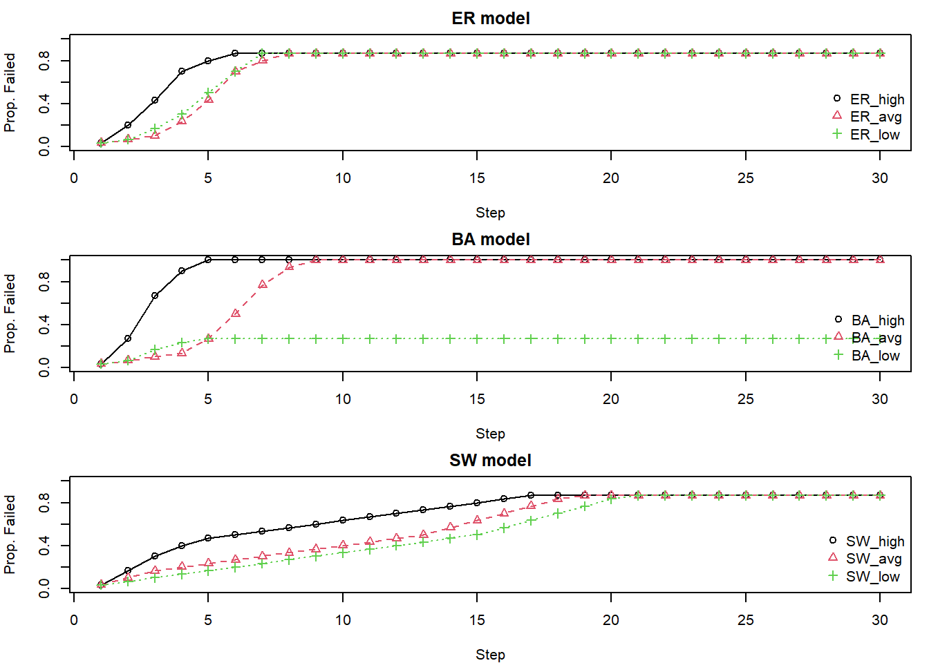
par(op)From the plots, you can see that for the ER and Small World models, nodes with high, average, low degree fail anyway just at different speeds. In the BA model, however, there is a distinctive difference between nodes with low degree and those with high & average degree. While the first two model represent homogeneous networks, the latter represents a heterogeneous one.
Define the CASCADE model for Cascading Failures
Dobson et al. (2007) proposed the CASCADE model, where cascading failures occur in terms of load exceeding a threshold and subsequent load redistribution.
Formally, CASCADE models are defined by selecting a graph with \(N\) vertices that each share a random load value. The minimum value of a given load is \(L^{\text{min}}\) and the maximum load is \(L^{\text{max}}\). For all \(N\) vertices, they are given an initial load, \(L_{j}\) which is distributed uniformly between \([L^{\text{min}}, L^{\text{max}}]\).
The normalized initial load for the \(j^{th}\) vertex is given by \(\ell_{j}\) where:
\[ \ell_{j} = \frac{L_{j} - L^{\text{min}}}{L^{\text{max}} - L^{\text{min}}} \] \(\ell_{j}\) is a random variable uniformly distributed on [0, 1].
Failure threshold: components fail when their load exceeds \(L^{\text{fail}}\)
Load transfer: The normalized load increment \(p\) is the amount of load increase on any component contingent on the failure of other components. It is expressed as a fraction of the load range \(L^{\text{max}} - L^{\text{min}}\)
\[ p = \frac{P}{L^{\text{max}} - L^{\text{min}}} \] \(d\) is a shifted initial disturbance expressed as a fraction of the load range
\[ d = \frac{D+L^{\text{max}} - L^{\text{min}}}{L^{\text{max}} - L^{\text{min}}} \] Following an initial disturbance \(D\) (where \(d\) is normalized \(D\)), components fail when their total load (\(L_{j} + D\)) exceeds the failure threshold (\(L^{\text{fail}}\)). Following each failure, an extra load of \(p\) is redistributed to the remaining components, though which the subsequent process may eventually lead to a global cascade.
Compare and Contrast Watts’ Cascades from the CASCADE Model
### "Complex" Xiang Cascade

cascade.Xiang = function(g, beta = 1, T = 1.2, alpha = 1, max.steps = 10000) {
  N = vcount(g)
  deg = igraph::degree(g)
  # Load is based on beta, alpha, and degree
  load0 = beta * (deg^alpha)
  cap = T * load0
  # Choose high, average, and lowest degree vertices
  high = which.max(deg)
  low = which.min(deg)
  avg = which.min(abs(deg - mean(deg)))[1]
  seeds = list(High=high, Average=avg, Low=low)
  results = lapply(seeds, function(seed) {
    load = load0
    failed = logical(N)
    # Kill the target
    # Find neighbors
    # Distribute failure to other neighbors
    # High degree neighbors take more load
    failed[seed] = TRUE
    nbrs = as.integer(neighbors(g,seed))
    if (length(nbrs)) {
      wts = deg[nbrs]^alpha
      load[nbrs] = load[nbrs] + load[seed]*(wts/sum(wts))
    }
    load[seed] = 0

    series = sum(failed)/N
    t = 1
    while (t < max.steps) {
      to_fail = which(!failed & (load > cap))
      if (!length(to_fail)) break
      for (v in to_fail) {
        failed[v] = TRUE
        nbrs2 = setdiff(as.integer(neighbors(g,v)), which(failed))
        if (length(nbrs2)) {
          w2 = deg[nbrs2]^alpha
          load[nbrs2] = load[nbrs2] + load[v]*(w2/sum(w2))
        }
        load[v] = 0
      }
      t = t+1
      series[t] = sum(failed)/N
    }
    series
  })

  names(results) = names(seeds)
  results
}


sim.funk = function(rep_id, n_nodes) {
  set.seed(15846 + rep_id)
  g_ba = sample_pa(n = n_nodes, power = 1, m = 2, directed = FALSE)
  g_er = sample_gnm(n = n_nodes, m = ecount(g_ba), directed = FALSE)
  g_sw = sample_smallworld(dim = 1, size = n_nodes, nei = floor(ecount(g_ba)/n_nodes), p = 0.05)
  ER.set = cascade.Xiang(g_er, beta = 1, T = 1.2, alpha = 1, max.steps = 1000)
  BA.set = cascade.Xiang(g_ba, beta = 1, T = 1.2, alpha = 1, max.steps = 1000)
  SW.set = cascade.Xiang(g_sw, beta = 1, T = 1.2, alpha = 1, max.steps = 1000)
  list(
    ER_high = ER.set$High,
    ER_avg  = ER.set$Average,
    ER_low  = ER.set$Low,
    BA_high = BA.set$High,
    BA_avg  = BA.set$Average,
    BA_low  = BA.set$Low,
    SW_high = SW.set$High,
    SW_avg  = SW.set$Average,
    SW_low  = SW.set$Low
  )
}
n_nodes = 30
results = sim.funk(34, n_nodes = n_nodes)
models = c("ER","BA","SW")
max_len = 30
op = par(mfrow=c(3,1), mar=c(4,4,2,1))

for(m in models) {
  idx = grep(paste0("^", m, "_"), names(results))
  raw = results[idx]
  mat = sapply(raw, function(v) {
    L = length(v)
    if (L < max_len) {
      c(v, rep(v[L], max_len - L))
    } else {
      v[1:max_len]
    }
  })

  matplot(1:max_len, mat,
          type = "o", pch = 1:3,
          col = 1:3, xlab = "Step",
          ylab = "Prop. Failed",
          main = paste(m, "model"),
          xlim = c(1, max_len),
          ylim = c(0, 1))
  legend("bottomright", legend = names(results)[idx],
         col = 1:3, pch = 1:3, bty = "n")
}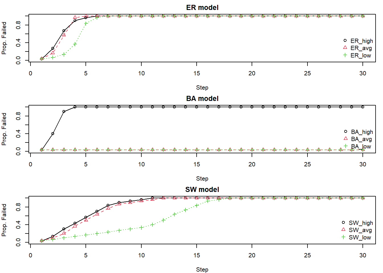
par(op)The Watt’s description is more simplistic, vertices have thresholds internal to themselves and are influenced entirely by neighbors. In the CASCADE model, vertices have resilience and an initial load such that they can exhibit more nuanced dynamics in how they fail.
While failures in Watt’s model depend almost entirely on the neighbors as the threshold hold is defined as the fraction of activated neighbors, the CASCADE model may allow us to consider resilience, as it introduces load and capacity whose gap will help contain failures to a small extent. Watts’ model also emphasizes the structure of networks represented as heterogeneous or homogeneous, where high or low connectivity leads to varying consequences.
Ash & Newth (2007) specified important topological properties that influence resilience of networks, which is about managing the redistribution of loads and consequent failures to control loads under capacity. The propertices are clustering, modularity, and path length. Higher modularity makes it possible to prevent failures from impacting the whole system by isolating local failures. Higher clustering could help maintain the stability of the network as alternative paths are available. Longer pathways could delay how rapidly an impact is delivered, allowing time for the disturbance to be resolved.
This emphasizes the importance of
- degree distribution, as it influences clustering and modularity
- topological properties such as betweenness centrality, to understand the importance of certain nodes alongside degree. In the iterative process of extending cascading failures, not only how many connections a node has but also where it is located in the network is decisive.
Do you remember Bringmann et al. (2019) concluded that betweenness centraility is not useful for measuring node importance for psychological networks? In the context of cascading failures, we could reach the opposite conclusion.
Can We Know the Thresholds for Vertices?
Thresholds could be influenced by internal or external factors. Even though we cannot completely separate thresholds from complex human behavior, there might be related concepts that could hint at the mechanisms of resilience, thresholds, and cascading failures.
What is a “threshold” for psychological vertices?
I tried to come up with some examples that are closer to psychological vertices and understand the threshold within their contexts.
For Watts’ model, which is rather straightforward, the closest example I could come up with is stress-related diarrhea.
- Stress exposure
- Cortisol + Adrenaline released
- Sympathetic nervous system activated
- Blood flow diverted away from digestive system
- Gut movement increases dramatically to empty gut to save energy
- Large intestine loses water absorption capacity
- Diarrhea
At each step, the threshold is whether the neighboring or mechanisms are activated or not.
For the CASCADE model, burnout might be a suitable example.
Burnout has three subdimensions: exhaustion, inefficacy, and cynicism. If we see burnout as a whole system failure, factors that influence the three dimensions carry loads that could activate each dimension. For example, exhaustion may be connected to health behavior, sleep patterns, and diet. Once stress causes a failure in sleep patterns, there is a possibility that it could trigger exhaustion. However, if health behavior and diet could share the load and absorb the stress, then a disturbance in sleep patterns might remain contained. In this context, the threshold is the difference between the capacity to handle disturbance and the total load that stress entails. A range of environmental and personal factors influence load, threshold, and capacity.
Weave in Graph Structures
Do you expect Erdős–Rényi and Barabási–Albert random graphs to exhibit different properties in their susceptibility to cascading failures? Why?
Since the former assumes a homogeneous network where load is redistributed to many similar neighbors rather than a few hubs, the impact may be contained at a local and modest level. On the other hand, BA random graphs represent heterogeneous networks whose degree distribution follows a power-law, assuming fewer high-degree nodes (hubs) and more low-degree ones. This could lead to rapid and global failures when the hubs are impacted.
For Barabási–Albert random graphs, do you expect the property of assortivity to come into play?
Disassortative networks benefit from the configuration where high-degree nodes tend to connect with low-degree nodes, creating more resilient structures. Redistributing the load to many low-degree nodes that are not heavily connected may slow the dispersion of failure and allow for more even load distribution.
The fact is, when real-world networks develop, they build in structural stability to be resilient to failure. Assortivity can be a tool for this. Explain.
Intuitively speaking, a high-degree node carrying a heavy load should be connected to low-degree nodes to ensure alternative paths and smooth load redistribution. Think of a few large cities carrying heavy traffic connected to smaller cities with lighter traffic. The overall traffic can still flow even when some roads are disconnected.
Discussion
As you may have noticed from the readings, cascading failure models tend to assume more physical or external interactions among agents such as humans, power stations, and organs. This may make it harder for psychologists interested in these models to implement them in ways that capture cascading failures.
What are the assumptions that distinguish psychological networks from the various networks discussed in the context of cascading failures?